versions/1.9.1/api/python/docs/_sources/tutorials/performance/backend/profiler.ipynb

{
 "cells": [
  {
   "cell_type": "markdown",
   "id": "16da8d35",
   "metadata": {},
   "source": [
    "<!--- Licensed to the Apache Software Foundation (ASF) under one -->\n",
    "<!--- or more contributor license agreements.  See the NOTICE file -->\n",
    "<!--- distributed with this work for additional information -->\n",
    "<!--- regarding copyright ownership.  The ASF licenses this file -->\n",
    "<!--- to you under the Apache License, Version 2.0 (the -->\n",
    "<!--- \"License\"); you may not use this file except in compliance -->\n",
    "<!--- with the License.  You may obtain a copy of the License at -->\n",
    "\n",
    "<!---   http://www.apache.org/licenses/LICENSE-2.0 -->\n",
    "\n",
    "<!--- Unless required by applicable law or agreed to in writing, -->\n",
    "<!--- software distributed under the License is distributed on an -->\n",
    "<!--- \"AS IS\" BASIS, WITHOUT WARRANTIES OR CONDITIONS OF ANY -->\n",
    "<!--- KIND, either express or implied.  See the License for the -->\n",
    "<!--- specific language governing permissions and limitations -->\n",
    "<!--- under the License. -->\n",
    "\n",
    "# Profiling MXNet Models\n",
    "\n",
    "It is often helpful to check the execution time of each operation in a neural network. You can then determine where to focus your effort to speed up model training or inference. In this tutorial, we will learn how to profile MXNet models to measure their running time and memory consumption using the MXNet profiler.\n",
    "\n",
    "## The incorrect way to profile\n",
    "\n",
    "If you have just started to use MXNet, you might be tempted to measure the execution time of your model using Python's `time` module like shown below:"
   ]
  },
  {
   "cell_type": "markdown",
   "id": "b1511b68",
   "metadata": {},
   "source": [
    "```python\n",
    "from time import time\n",
    "from mxnet import autograd, nd\n",
    "import mxnet as mx\n",
    "\n",
    "start = time()\n",
    "x = nd.random_uniform(shape=(2000,2000))\n",
    "y = nd.dot(x, x)\n",
    "print('Time for matrix multiplication: %f sec\\n' % (time() - start))\n",
    "\n",
    "start = time()                                \n",
    "y_np = y.asnumpy()                             \n",
    "print('Time for converting to numpy: %f sec' % (time() - start))\n",
    "```\n"
   ]
  },
  {
   "cell_type": "markdown",
   "id": "3c99f44a",
   "metadata": {},
   "source": [
    "**Time for matrix multiplication: 0.005051 sec**<!--notebook-skip-line-->\n",
    "\n",
    "**Time for converting to numpy: 0.167693 sec**<!--notebook-skip-line-->\n",
    "\n",
    "From the timings above, it seems as if converting to numpy takes lot more time than multiplying two large matrices. That doesn't seem right.\n",
    "\n",
    "This is because, in MXNet, all operations are executed asynchronously. So, when `nd.dot(x, x)` returns, the matrix multiplication is not complete, it has only been queued for execution. However, [asnumpy](https://mxnet.apache.org/api/python/ndarray/ndarray.html?highlight=asnumpy#mxnet.ndarray.NDArray.asnumpy) has to wait for the result to be calculated in order to convert it to numpy array on CPU, hence taking a longer time. Other examples of 'blocking' operations include [asscalar](https://mxnet.apache.org/api/python/ndarray/ndarray.html?highlight=asscalar#mxnet.ndarray.NDArray.asscalar) and [wait_to_read](https://mxnet.apache.org/api/python/ndarray/ndarray.html?highlight=wait_to_read#mxnet.ndarray.NDArray.wait_to_read).\n",
    "\n",
    "While it is possible to use [NDArray.waitall()](https://mxnet.apache.org/api/python/ndarray/ndarray.html?highlight=waitall#mxnet.ndarray.waitall) before and after operations to get running time of operations, it is not a scalable method to measure running time of multiple sets of operations, especially in a [Sequential](https://mxnet.apache.org/api/python/gluon/gluon.html?highlight=sequential#mxnet.gluon.nn.Sequential) or hybridized network.\n",
    "\n",
    "## The correct way to profile\n",
    "\n",
    "The correct way to measure running time of MXNet models is to use MXNet profiler. In the rest of this tutorial, we will learn how to use the MXNet profiler to measure the running time and memory consumption of MXNet models. You can import the profiler and configure it from Python code."
   ]
  },
  {
   "cell_type": "markdown",
   "id": "875c06c3",
   "metadata": {},
   "source": [
    "```python\n",
    "from mxnet import profiler\n",
    "\n",
    "profiler.set_config(profile_all=True,\n",
    "                    aggregate_stats=True,\n",
    "                    continuous_dump=True,\n",
    "                    filename='profile_output.json')\n",
    "```\n"
   ]
  },
  {
   "cell_type": "markdown",
   "id": "e021b27e",
   "metadata": {},
   "source": [
    "`profile_all` enables all types of profiling. You can also individually enable the following types of profiling:\n",
    "\n",
    "- `profile_symbolic` (boolean): whether to profile symbolic operators\n",
    "- `profile_imperative` (boolean): whether to profile imperative operators\n",
    "- `profile_memory` (boolean): whether to profile memory usage\n",
    "- `profile_api` (boolean): whether to profile the C API\n",
    "\n",
    "`aggregate_stats` aggregates statistics in memory which can then be printed to console by calling `profiler.dumps()`.\n",
    "\n",
    "### Setup: Build a model\n",
    "\n",
    "Let's build a small convolutional neural network that we can use to demonstrate profiling."
   ]
  },
  {
   "cell_type": "markdown",
   "id": "cae117d8",
   "metadata": {},
   "source": [
    "```python\n",
    "from mxnet import gluon\n",
    "\n",
    "net = gluon.nn.HybridSequential()\n",
    "with net.name_scope():\n",
    "    net.add(gluon.nn.Conv2D(channels=20, kernel_size=5, activation='relu'))\n",
    "    net.add(gluon.nn.MaxPool2D(pool_size=2, strides=2))\n",
    "    net.add(gluon.nn.Conv2D(channels=50, kernel_size=5, activation='relu'))\n",
    "    net.add(gluon.nn.MaxPool2D(pool_size=2, strides=2))\n",
    "    net.add(gluon.nn.Flatten())\n",
    "    net.add(gluon.nn.Dense(512, activation=\"relu\"))\n",
    "    net.add(gluon.nn.Dense(10))\n",
    "```\n"
   ]
  },
  {
   "cell_type": "markdown",
   "id": "6357f35c",
   "metadata": {},
   "source": [
    "We need data that we can run through the network for profiling. We'll use the MNIST dataset."
   ]
  },
  {
   "cell_type": "markdown",
   "id": "30d1f46d",
   "metadata": {},
   "source": [
    "```python\n",
    "from mxnet.gluon.data.vision import transforms\n",
    "\n",
    "dataset = gluon.data.vision.MNIST(train=True)\n",
    "dataset = dataset.transform_first(transforms.ToTensor())\n",
    "dataloader = gluon.data.DataLoader(dataset, batch_size=64, shuffle=True)\n",
    "```\n"
   ]
  },
  {
   "cell_type": "markdown",
   "id": "1394fba4",
   "metadata": {},
   "source": [
    "Let's define a function that will run a single training iteration given `data` and `label`."
   ]
  },
  {
   "cell_type": "markdown",
   "id": "86b0d0fe",
   "metadata": {},
   "source": [
    "```python\n",
    "# Use GPU if available\n",
    "if mx.context.num_gpus():\n",
    "    ctx=mx.gpu()\n",
    "else:\n",
    "    ctx=mx.cpu()\n",
    "\n",
    "# Initialize the parameters with random weights\n",
    "net.collect_params().initialize(mx.init.Xavier(), ctx=ctx)\n",
    "\n",
    "# Use SGD optimizer\n",
    "trainer = gluon.Trainer(net.collect_params(), 'sgd', {'learning_rate': 0.1})\n",
    "\n",
    "# Softmax Cross Entropy is a frequently used loss function for multi-class classification\n",
    "softmax_cross_entropy = gluon.loss.SoftmaxCrossEntropyLoss()\n",
    "\n",
    "# A helper function to run one training iteration\n",
    "def run_training_iteration(data, label):\n",
    "    # Load data and label is the right context\n",
    "    data = data.as_in_context(ctx)\n",
    "    label = label.as_in_context(ctx)\n",
    "    # Run the forward pass\n",
    "    with autograd.record():\n",
    "        output = net(data)\n",
    "        loss = softmax_cross_entropy(output, label)\n",
    "    # Run the backward pass\n",
    "    loss.backward()\n",
    "    # Apply changes to parameters\n",
    "    trainer.step(data.shape[0])\n",
    "```\n"
   ]
  },
  {
   "cell_type": "markdown",
   "id": "3df8fe20",
   "metadata": {},
   "source": [
    "### Starting and stopping the profiler from Python\n",
    "\n",
    "When the first forward pass is run on a network, MXNet does a number of housekeeping tasks including inferring the shapes of various parameters, allocating memory for intermediate and final outputs, etc. For these reasons, profiling the first iteration doesn't provide representative results for the rest of training. We will, therefore, skip the first iteration."
   ]
  },
  {
   "cell_type": "markdown",
   "id": "45e2cde8",
   "metadata": {},
   "source": [
    "```python\n",
    "# Run the first iteration without profiling\n",
    "itr = iter(dataloader)\n",
    "run_training_iteration(*next(itr))\n",
    "```\n"
   ]
  },
  {
   "cell_type": "markdown",
   "id": "b5cbb851",
   "metadata": {},
   "source": [
    "We'll run the next iteration with the profiler turned on."
   ]
  },
  {
   "cell_type": "markdown",
   "id": "bf8f0efe",
   "metadata": {},
   "source": [
    "```python\n",
    "data, label = next(itr)\n",
    "\n",
    "# Ask the profiler to start recording\n",
    "profiler.set_state('run')\n",
    "\n",
    "run_training_iteration(*next(itr))\n",
    "\n",
    "# Make sure all operations have completed\n",
    "mx.nd.waitall()\n",
    "# Ask the profiler to stop recording\n",
    "profiler.set_state('stop')\n",
    "# Dump all results to log file before download\n",
    "profiler.dump()\n",
    "```\n"
   ]
  },
  {
   "cell_type": "markdown",
   "id": "839a7389",
   "metadata": {},
   "source": [
    "Between running and stopping the profiler, you can also pause and resume the profiler using `profiler.pause()` and `profiler.resume()` respectively to profile only parts of the code you want to profile.\n",
    "\n",
    "### Starting the profiler automatically using an environment variable\n",
    "\n",
    "The method described above requires code changes to start and stop the profiler. You can also start the profiler automatically and profile the entire code without any code changes using the `MXNET_PROFILER_AUTOSTART` environment variable.\n",
    "\n",
    "`$ MXNET_PROFILER_AUTOSTART=1 python my_script.py`\n",
    "\n",
    "MXNet will start the profiler automatically if you run your code with the environment variable `MXNET_PROFILER_AUTOSTART` set to `1`. The profiler output is stored in `profile.json` inside the current directory.\n",
    "\n",
    "Note that the profiler output could be large depending on your code. It might be helpful to profile only sections of your code using the `set_state` API described in the previous section.\n",
    "\n",
    "### Increasing granularity of the profiler output\n",
    "\n",
    "MXNet executes computation graphs in 'bulk mode' which reduces kernel launch gaps in between symbolic operators for faster execution. This could reduce the granularity of the profiler output. If you need profiling result of every operator, please set the environment variables `MXNET_EXEC_BULK_EXEC_INFERENCE` and `MXNET_EXEC_BULK_EXEC_TRAIN` to `0` to disable the bulk execution mode.\n",
    "\n",
    "When working with networks created using the Gluon API, you will get a more granular profiling outputs if you profile networks that haven't been hybridized. Operations can appear fused together in the profiling outputs after hybridization, which can make debugging tricky.\n",
    "\n",
    "### Viewing profiler output\n",
    "\n",
    "There are a few ways to view the information collected by the profiler. You can view it in the console, you can view a more graphical version in a browser, or you can use a vendor tool such as Intel VTune or Nvidia NVProf to view output. For most scenarios the information you need can be obtained with MXNet's built in profiler support, but if you want to investigate the performance of operators alongside extra context about your hardware (e.g. cache hit rates, or CUDA kernel timings) then profiling jointly with vendor tools is recommended.\n",
    "\n",
    "#### 1. View in console\n",
    "\n",
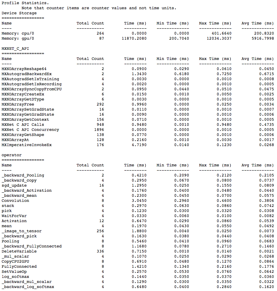
    "You can use the `profiler.dumps()` method to view the information collected by the profiler in the console. The collected information contains time taken by each operator, time taken by each C API and memory consumed in both CPU and GPU."
   ]
  },
  {
   "cell_type": "markdown",
   "id": "b019f35c",
   "metadata": {},
   "source": [
    "```python\n",
    "profiler.set_state('run')\n",
    "profiler.set_state('stop')\n",
    "print(profiler.dumps())\n",
    "```\n"
   ]
  },
  {
   "cell_type": "markdown",
   "id": "2c07dd9e",
   "metadata": {},
   "source": [
    "![Profile Statistics](https://raw.githubusercontent.com/dmlc/web-data/master/mxnet/tutorials/python/profiler/profile_stats.png)<!--notebook-skip-line-->\n",
    "\n",
    "#### 2. View in browser\n",
    "\n",
    "You can also dump the information collected by the profiler into a `json` file using the `profiler.dump()` function and view it in a browser."
   ]
  },
  {
   "cell_type": "markdown",
   "id": "e4dafe36",
   "metadata": {},
   "source": [
    "```python\n",
    "profiler.dump(finished=False)\n",
    "```\n"
   ]
  },
  {
   "cell_type": "markdown",
   "id": "eaa8cb70",
   "metadata": {},
   "source": [
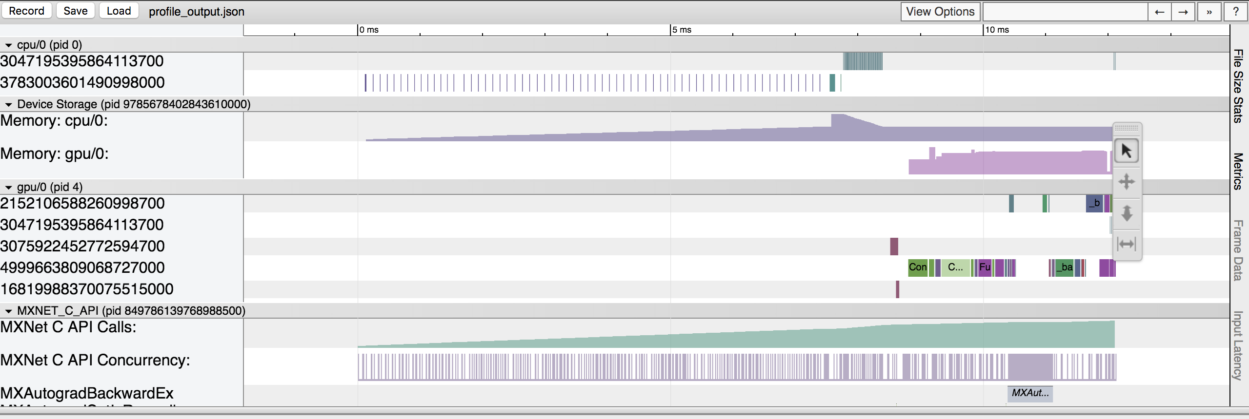
    "`dump()` creates a `json` file which can be viewed using a trace consumer like `chrome://tracing` in the Chrome browser. Here is a snapshot that shows the output of the profiling we did above. Note that setting the `finished` parameter to `False` will prevent the profiler from finishing dumping to file. If you just use `profiler.dump()`, you will no longer be able to profile the remaining sections of your model. \n",
    "\n",
    "![Tracing Screenshot](https://raw.githubusercontent.com/dmlc/web-data/master/mxnet/tutorials/python/profiler/profiler_output_chrome.png)\n",
    "\n",
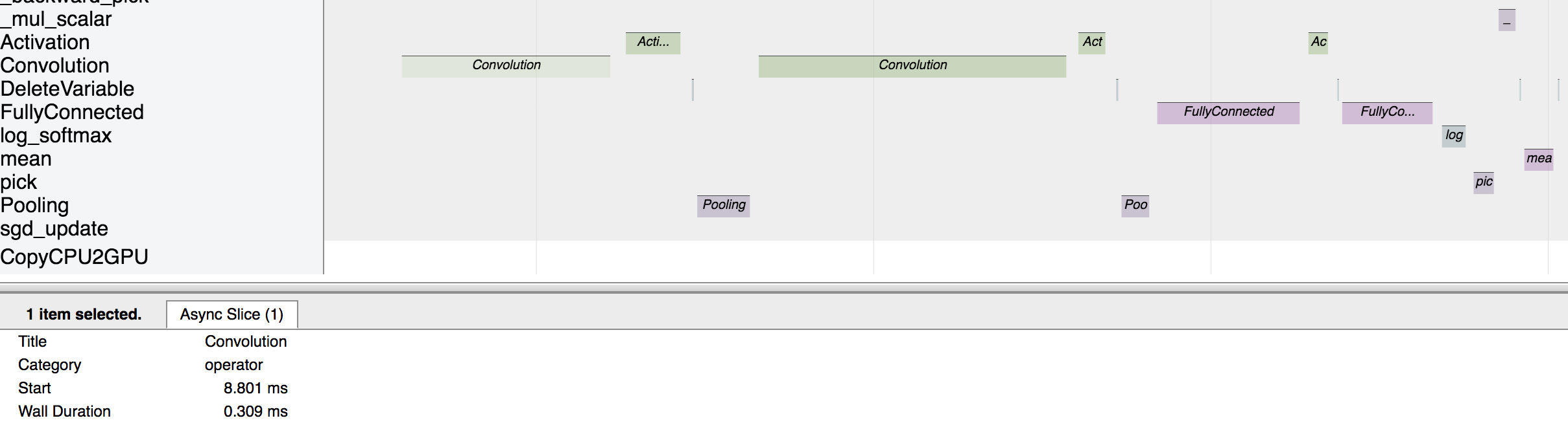
    "Let's zoom in to check the time taken by operators\n",
    "\n",
    "![Operator profiling](https://raw.githubusercontent.com/dmlc/web-data/master/mxnet/tutorials/python/profiler/profile_operators.png)\n",
    "\n",
    "The above picture visualizes the sequence in which the operators were executed and the time taken by each operator.\n",
    "\n",
    "### Profiling MKLDNN Operators\n",
    "Reagrding MKLDNN operators, the library has already provided the internal profiling tool. Firstly, you need set `MKLDNN_VERBOSE=1` to enable internal profiler.\n",
    "\n",
    "`$ MKLDNN_VERBOSE=1 python my_script.py > mkldnn_verbose.log`\n",
    "\n",
    "Now, the detailed profiling insights of each mkldnn prmitive are saved into `mkldnn_verbose.log` (like below)."
   ]
  },
  {
   "cell_type": "markdown",
   "id": "7d1004bc",
   "metadata": {},
   "source": [
    "```\n",
    "dnnl_verbose,info,DNNL v1.1.2 (commit cb2cc7ac17ff4e2ef50805c7048d33256d82be4d)\n",
    "dnnl_verbose,info,Detected ISA is Intel AVX-512 with Intel DL Boost\n",
    "dnnl_verbose,exec,cpu,convolution,jit:avx512_common,forward_inference,src_f32::blocked:aBcd16b:f0 wei_f32::blocked:ABcd16b16a:f0 bia_undef::undef::f0 dst_f32::blocked:aBcd16b:f0,,alg:convolution_direct,mb32_ic32oc32_ih256oh256kh3sh1dh0ph1_iw256ow256kw3sw1dw0pw1,20.7539\n",
    "```\n"
   ]
  },
  {
   "cell_type": "markdown",
   "id": "269bde5f",
   "metadata": {},
   "source": [
    "For example, if you want to calculate the total executing time of `convolution` primitive, you can just run:\n",
    "\n",
    "`$ cat mkldnn_verbose.log | grep \"exec,cpu,convolution\" | awk 'BEGIN{FS=\",\"} {SUM+=$11} END {print SUM}'`\n",
    "\n",
    "Moreover, you can set `MKLDNN_VERBOSE=2` to collect both creating and executing time of each primitive.\n",
    "\n",
    "`$ cat mkldnn_verbose.log | grep \"create,cpu,convolution\" | awk 'BEGIN{FS=\",\"} {SUM+=$11} END {print SUM}'`\n",
    "\n",
    "`$ cat mkldnn_verbose.log | grep \"exec,cpu,convolution\" | awk 'BEGIN{FS=\",\"} {SUM+=$11} END {print SUM}'`\n",
    "\n",
    "\n",
    "### Profiling Custom Operators\n",
    "Should the existing NDArray operators fail to meet all your model's needs, MXNet supports [Custom Operators](/api/python/docs/tutorials/extend/customop.html) that you can define in Python. In `forward()` and `backward()` of a custom operator, there are two kinds of code: \"pure Python\" code (NumPy operators included) and \"sub-operators\" (NDArray operators called within `forward()` and `backward()`). With that said, MXNet can profile the execution time of both kinds without additional setup. Specifically, the MXNet profiler will break a single custom operator call into a pure Python event and several sub-operator events if there are any. Furthermore, all of those events will have a prefix in their names, which is, conveniently, the name of the custom operator you called.\n",
    "\n",
    "Let's try profiling custom operators with the following code example:"
   ]
  },
  {
   "cell_type": "markdown",
   "id": "b37c6ad9",
   "metadata": {},
   "source": [
    "```python\n",
    "class MyAddOne(mx.operator.CustomOp):\n",
    "    def forward(self, is_train, req, in_data, out_data, aux):  \n",
    "        self.assign(out_data[0], req[0], in_data[0]+1)\n",
    "\n",
    "    def backward(self, req, out_grad, in_data, out_data, in_grad, aux):\n",
    "        self.assign(in_grad[0], req[0], out_grad[0])\n",
    "\n",
    "@mx.operator.register('MyAddOne')\n",
    "class CustomAddOneProp(mx.operator.CustomOpProp):\n",
    "    def __init__(self):\n",
    "        super(CustomAddOneProp, self).__init__(need_top_grad=True)\n",
    "\n",
    "    def list_arguments(self):\n",
    "        return ['data']\n",
    "\n",
    "    def list_outputs(self):\n",
    "        return ['output']\n",
    "\n",
    "    def infer_shape(self, in_shape):\n",
    "        return [in_shape[0]], [in_shape[0]], []\n",
    "\n",
    "    def create_operator(self, ctx, shapes, dtypes):\n",
    "        return MyAddOne()\n",
    "\n",
    "\n",
    "inp = mx.nd.zeros(shape=(500, 500))\n",
    "\n",
    "profiler.set_config(profile_all=True, continuous_dump=True, \\\n",
    "                    aggregate_stats=True)\n",
    "profiler.set_state('run')\n",
    "\n",
    "w = nd.Custom(inp, op_type=\"MyAddOne\")\n",
    "\n",
    "mx.nd.waitall()\n",
    "\n",
    "profiler.set_state('stop')\n",
    "print(profiler.dumps())\n",
    "profiler.dump(finished=False)\n",
    "```\n"
   ]
  },
  {
   "cell_type": "markdown",
   "id": "1efbcfec",
   "metadata": {},
   "source": [
    "Here, we have created a custom operator called `MyAddOne`, and within its `forward()` function, we simply add one to the input. We can visualize the dump file in `chrome://tracing/`:\n",
    "\n",
    "![Custom Operator Profiling Screenshot](https://raw.githubusercontent.com/dmlc/web-data/master/mxnet/tutorials/python/profiler/profiler_output_custom_operator_chrome.png)\n",
    "\n",
    "As shown by the screenshot, in the **Custom Operator** domain where all the custom operator-related events fall into, we can easily visualize the execution time of each segment of `MyAddOne`. We can tell that `MyAddOne::pure_python` is executed first. We also know that `CopyCPU2CPU` and `_plus_scalr` are two \"sub-operators\" of `MyAddOne` and the sequence in which they are executed.\n",
    "\n",
    "Please note that: to be able to see the previously described information, you need to set `profile_imperative` to `True` even when you are using custom operators in [symbolic mode](https://mxnet.apache.org/versions/master/tutorials/basic/symbol.html) (refer to the code snippet below, which is the symbolic-mode equivelent of the code example above). The reason is that within custom operators, pure python code and sub-operators are still called imperatively."
   ]
  },
  {
   "cell_type": "markdown",
   "id": "957b5ab9",
   "metadata": {},
   "source": [
    "```python \n",
    "# Set profile_all to True\n",
    "profiler.set_config(profile_all=True, aggregate_stats=True, continuous_dump=True)\n",
    "# OR, Explicitly Set profile_symbolic and profile_imperative to True\n",
    "profiler.set_config(profile_symbolic=True, profile_imperative=True, \\\n",
    "                    aggregate_stats=True, continuous_dump=True)\n",
    "\n",
    "profiler.set_state('run')\n",
    "# Use Symbolic Mode\n",
    "a = mx.symbol.Variable('a')\n",
    "b = mx.symbol.Custom(data=a, op_type='MyAddOne')\n",
    "c = b.bind(mx.cpu(), {'a': inp})\n",
    "y = c.forward()\n",
    "mx.nd.waitall()\n",
    "profiler.set_state('stop')\n",
    "print(profiler.dumps())\n",
    "profiler.dump()\n",
    "```\n"
   ]
  },
  {
   "cell_type": "markdown",
   "id": "4d8e4a48",
   "metadata": {},
   "source": [
    "### Some Rules to Pay Attention to\n",
    "1. Always use `profiler.dump(finished=False)` if you do not intend to finish dumping to file. Otherwise, calling `profiler.dump()` in the middle of your model may lead to unexpected behaviors; and if you subsequently call `profiler.set_config()`, the program will error out.\n",
    "\n",
    "2. You can only dump to one file. Do not change the target file by calling `profiler.set_config(filename='new_name.json')` in the middle of your model. This will lead to incomplete dump outputs.\n",
    "\n",
    "## Advanced: Using NVIDIA Profiling Tools\n",
    "\n",
    "MXNet's Profiler is the recommended starting point for profiling MXNet code, but NVIDIA also provides a couple of tools for low-level profiling of CUDA code: [NVProf](https://devblogs.nvidia.com/cuda-pro-tip-nvprof-your-handy-universal-gpu-profiler/), [Visual Profiler](https://developer.nvidia.com/nvidia-visual-profiler) and [Nsight Compute](https://developer.nvidia.com/nsight-compute). You can use these tools to profile all kinds of executables, so they can be used for profiling Python scripts running MXNet. And you can use these in conjunction with the MXNet Profiler to see high-level information from MXNet alongside the low-level CUDA kernel information.\n",
    "\n",
    "#### NVProf and Visual Profiler\n",
    "\n",
    "NVProf and Visual Profiler are available in CUDA 9 and CUDA 10 toolkits. You can get a timeline view of CUDA kernel executions, and also analyse the profiling results to get automated recommendations. It is useful for profiling end-to-end training but the interface can sometimes become slow and unresponsive.\n",
    "\n",
    "You can initiate the profiling directly from inside Visual Profiler or from the command line with `nvprof` which wraps the execution of your Python script. If it's not on your path already, you can find `nvprof` inside your CUDA directory. See [this discussion post](https://discuss.mxnet.io/t/using-nvidia-profiling-tools-visual-profiler-and-nsight-compute/) for more details on setup.\n",
    "\n",
    "`$ nvprof -o my_profile.nvvp python my_profiler_script.py`\n",
    "\n",
    "`==11588== NVPROF is profiling process 11588, command: python my_profiler_script.py`\n",
    "\n",
    "`==11588== Generated result file: /home/user/Development/mxnet/ci/my_profile.nvvp`\n",
    "\n",
    "We specified an output file called `my_profile.nvvp` and this will be annotated with NVTX ranges (for MXNet operations) that will be displayed alongside the standard NVProf timeline. This can be very useful when you're trying to find patterns between operators run by MXNet, and their associated CUDA kernel calls.\n",
    "\n",
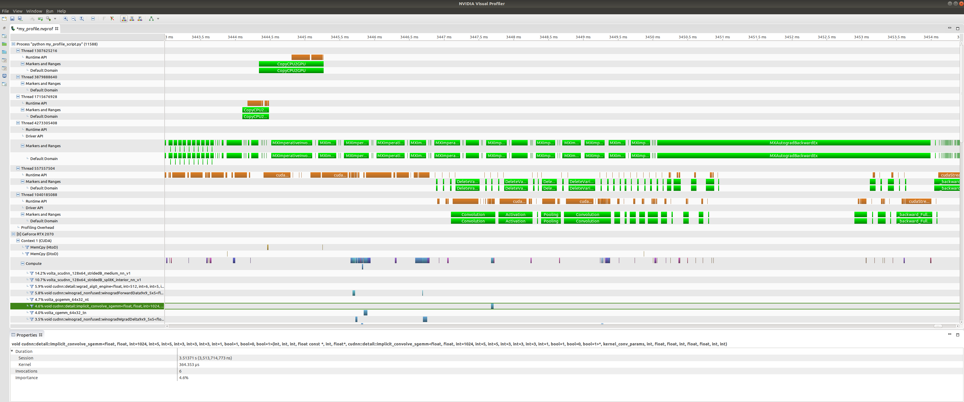
    "You can open this file in Visual Profiler to visualize the results.\n",
    "\n",
    "![Operator profiling](https://raw.githubusercontent.com/dmlc/web-data/master/mxnet/tutorials/python/profiler/profiler_nvprof.png)\n",
    "\n",
    "At the top of the plot we have CPU tasks such as driver operations, memory copy calls, MXNet engine operator invocations, and imperative MXNet API calls.  Below we see the kernels active on the GPU during the same time period.\n",
    "\n",
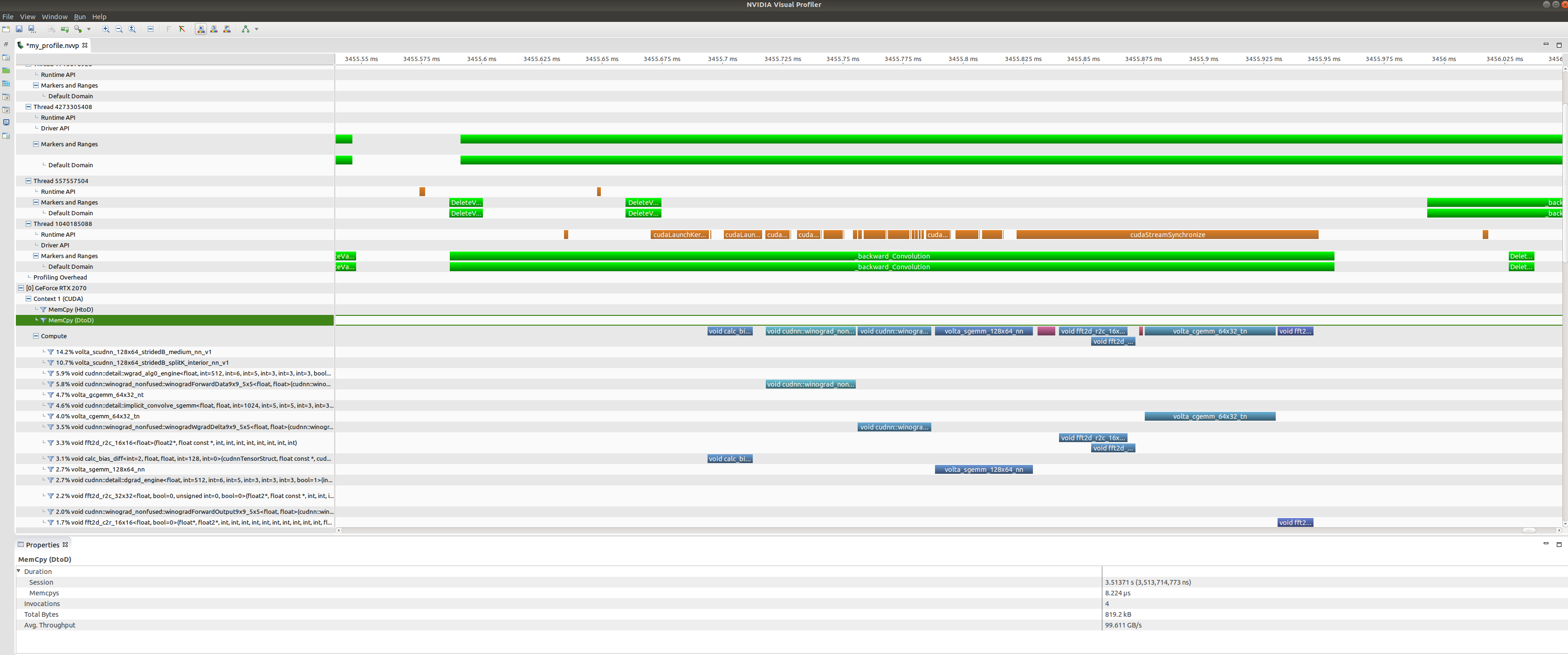    "![Operator profiling](https://raw.githubusercontent.com/dmlc/web-data/master/mxnet/tutorials/python/profiler/profiler_nvprof_zoomed.png)\n",
    "\n",
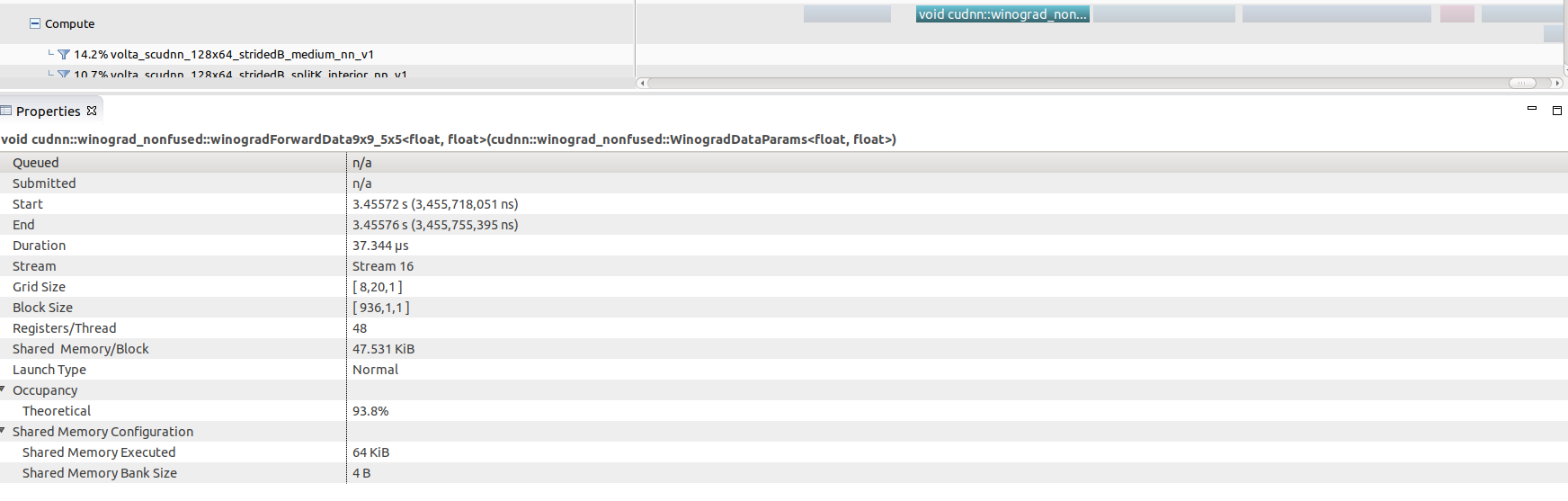
    "Zooming in on a backwards convolution operator we can see that it is in fact made up of a number of different GPU kernel calls, including a cuDNN winograd convolution call, and a fast-fourier transform call.\n",
    "\n",
    "![Operator profiling](https://raw.githubusercontent.com/dmlc/web-data/master/mxnet/tutorials/python/profiler/profiler_winograd.png)\n",
    "\n",
    "Selecting any of these kernel calls (the winograd convolution call shown here) will get you some interesting GPU performance information such as occupancy rates (vs theoretical), shared memory usage and execution duration.\n",
    "\n",
    "#### Nsight Compute\n",
    "\n",
    "Nsight Compute is available in CUDA 10 toolkit, but can be used to profile code running CUDA 9. You don't get a timeline view, but you get many low level statistics about each individual kernel executed and can compare multiple runs (i.e. create a baseline).\n",
    "\n",
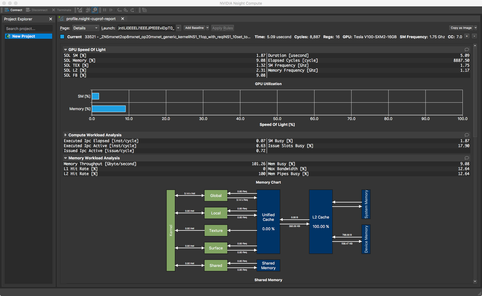    "![Nsight Compute](https://raw.githubusercontent.com/dmlc/web-data/master/mxnet/tutorials/python/profiler/profile_nsight_compute.png)\n",
    "\n",
    "### Further reading\n",
    "\n",
    "- [Examples using MXNet profiler.](https://github.com/apache/mxnet/tree/master/example/profiler)\n",
    "- [Some tips for improving MXNet performance.](https://mxnet.apache.org/api/faq/perf)\n",
    "\n",
    "<!-- INSERT SOURCE DOWNLOAD BUTTONS -->"
   ]
  }
 ],
 "metadata": {
  "language_info": {
   "name": "python"
  }
 },
 "nbformat": 4,
 "nbformat_minor": 5
}