| { |
| "cells": [ |
| { |
| "cell_type": "markdown", |
| "id": "48fa8141", |
| "metadata": {}, |
| "source": [ |
| "<!--- Licensed to the Apache Software Foundation (ASF) under one -->\n", |
| "<!--- or more contributor license agreements. See the NOTICE file -->\n", |
| "<!--- distributed with this work for additional information -->\n", |
| "<!--- regarding copyright ownership. The ASF licenses this file -->\n", |
| "<!--- to you under the Apache License, Version 2.0 (the -->\n", |
| "<!--- \"License\"); you may not use this file except in compliance -->\n", |
| "<!--- with the License. You may obtain a copy of the License at -->\n", |
| "\n", |
| "<!--- http://www.apache.org/licenses/LICENSE-2.0 -->\n", |
| "\n", |
| "<!--- Unless required by applicable law or agreed to in writing, -->\n", |
| "<!--- software distributed under the License is distributed on an -->\n", |
| "<!--- \"AS IS\" BASIS, WITHOUT WARRANTIES OR CONDITIONS OF ANY -->\n", |
| "<!--- KIND, either express or implied. See the License for the -->\n", |
| "<!--- specific language governing permissions and limitations -->\n", |
| "<!--- under the License. -->\n", |
| "\n", |
| "# Automatic Differentiation\n", |
| "\n", |
| "## Why do we need to calculate gradients?\n", |
| "\n", |
| "### Short Answer:\n", |
| "\n", |
| "Gradients are fundamental to the process of training neural networks, and tell us how to change the parameters of the network to improve its performance.\n", |
| "\n", |
| "\n", |
| "\n", |
| "### Long Answer:\n", |
| "\n", |
| "Under the hood, neural networks are composed of operators (e.g. sums, products, convolutions, etc) some of which use parameters (e.g. the weights in convolution kernels) for their computation, and it's our job to find the optimal values for these parameters. Gradients lead us to the solution!\n", |
| "\n", |
| "Gradients tell us how much a given variable increases or decreases when we change a variable it depends on. What we're interested in is the effect of changing a each parameter on the performance of the network. We usually define performance using a loss metric that we try to minimize, i.e. a metric that tells us how bad the predictions of a network are given ground truth. As an example, for regression we might try to minimize the [L2 loss](../../../api/gluon/loss/index.rst#mxnet.gluon.loss.L2Loss) (also known as the Euclidean distance) between our predictions and true values, and for classification we minimize the [cross entropy loss](../../../api/gluon/loss/index.rst#mxnet.gluon.loss.SoftmaxCrossEntropyLoss).\n", |
| "\n", |
| "Assuming we've calculated the gradient of each parameter with respect to the loss (details in next section), we can then use an optimizer such as [stochastic gradient descent](https://en.wikipedia.org/wiki/Stochastic_gradient_descent) to shift the parameters slightly in the *opposite direction* of the gradient. See [Optimizers](../../../api/optimizer/index.rst) for more information on these methods. We repeat the process of calculating gradients and updating parameters over and over again, until the parameters of the network start to stabilize and converge to a good solution.\n", |
| "\n", |
| "## How do we calculate gradients?\n", |
| "\n", |
| "### Short Answer:\n", |
| "\n", |
| "We differentiate. [MXNet Gluon](../gluon/index.ipynb) uses Reverse Mode Automatic Differentiation (`autograd`) to backprogate gradients from the loss metric to the network parameters.\n", |
| "\n", |
| "\n", |
| "\n", |
| "### Long Answer:\n", |
| "\n", |
| "One option would be to get out our calculus books and work out the gradients by hand. Who wants to do this though? It's time consuming and error prone for starters. Another option is [symbolic differentiation](https://www.cs.utexas.edu/users/novak/asg-symdif.html), which calculates the formulas for each gradient, but this quickly leads to incredibly long formulas as networks get deeper and operators get more complex. We could use finite differencing, and try slight differences on each parameter and see how the loss metric responds, but this is computationally expensive and can have poor [numerical precision](https://en.wikipedia.org/wiki/Finite_difference_coefficient).\n", |
| "\n", |
| "What's the solution? Use automatic differentiation to backpropagate the gradients from the loss metric back to each of the parameters. With [backpropagation](https://en.wikipedia.org/wiki/Backpropagation), a dynamic programming approach is taken to efficently calculate gradients. Sometimes this is called reverse mode automatic differentiation, and it's very efficient in 'fan-in' situations where many parameters effect a single loss metric. Although forward mode automatic differentiation methods exist, they're suited to 'fan-out' situations where few parameters effect many metrics, which isn't the case for training neural networks.\n", |
| "\n", |
| "## How does Automatic Differentiation (`autograd`) work?\n", |
| "\n", |
| "### Short Answer:\n", |
| "\n", |
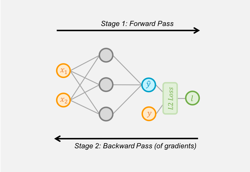
| "Stage 1. Create a record of the operators used by the network to make predictions and calculate the loss metric. Called the 'forward pass' of training.\n", |
| "Stage 2. Work backwards through this record and evaluate the partial derivatives of each operator, all the way back to the network parameters. Called the 'backward pass' of training.\n", |
| "\n", |
| "<p style=\"text-align:center\">\n", |
| " <video width=\"600\" controls playsinline autoplay muted loop>\n", |
| " <source src=\"/api/python/docs/_static/autograd_images/autograd_graph.mp4\" type=\"video/mp4\">\n", |
| " </video>\n", |
| "</p>\n", |
| "\n", |
| "### Long Answer:\n", |
| "\n", |
| "All operators in MXNet have two methods defined: a `forward` method for executing the operator as expected, and a `backward` method that returns the partial derivative (the derivative of the output with respect to the input). On the vary rare occasion you need to implement your own custom operator, you'll define the same two methods.\n", |
| "\n", |
| "Automatic differentiation creates a record of the operators used (i.e. the `forward` method calls) by the network to make predictions and calculate the loss metric. A graph structure is used to record this, capturing the inputs (including their value) and outputs for each operator and how the operators are related. We call this the 'forward pass' of training.\n", |
| "\n", |
| "Automatic differentiation then works backwards through each operator of the graph, calling the `backward` method on each operator to calculate the partial derivative and calculate the gradient of the loss metric with respect to the operator's input (which could be parameters). Usually we work backwards from the loss metric, and hence calculate the gradients of the loss metric, but this can be done from any output. We call this the 'backward pass' of training.\n", |
| "\n", |
| "## What are the advantages of Automatic Differentiation (`autograd`)?\n", |
| "\n", |
| "### Short Answer:\n", |
| "\n", |
| "It's flexible, automatic and efficient. You can use native Python control flow operators such as `if` conditions and `while` loops and `autograd` will still be able to backpropogate the gradients correctly.\n", |
| "\n", |
| "### Long Answer:\n", |
| "\n", |
| "A huge benefit of using `autograd` is the flexibility it gives you when defining your network. You can change the operations on every iteration, and `autograd` will still be able to backpropogate the gradients correctly. You'll sometimes hear these called 'dynamic graphs', and are much more complex to implement in frameworks that require static graphs, such as TensorFlow.\n", |
| "\n", |
| "As suggested by the name, `autograd` is automatic and so the complexities of the backpropogation procedure are taken care of for you. All you have to do is tell `autograd` when you're interested in recording gradients, and specify what gradients you're interested in calculating: this will nearly always just be the gradient of the loss metric. And these gradient calculations will be performed efficiently too.\n", |
| "\n", |
| "## How do I use `autograd` in MXNet Gluon?\n", |
| "\n", |
| "Step one is to import the `autograd` package." |
| ] |
| }, |
| { |
| "cell_type": "code", |
| "execution_count": 1, |
| "id": "1de18f6f", |
| "metadata": {}, |
| "outputs": [], |
| "source": [ |
| "from mxnet import autograd" |
| ] |
| }, |
| { |
| "cell_type": "markdown", |
| "id": "a31c2295", |
| "metadata": {}, |
| "source": [ |
| "As a simple example, we'll implement the regression model shown in the diagrams above, and later use `autograd` to automatically calculate the gradient of the loss with respect to each of the weight parameters." |
| ] |
| }, |
| { |
| "cell_type": "code", |
| "execution_count": 2, |
| "id": "3ea6b6b2", |
| "metadata": {}, |
| "outputs": [ |
| { |
| "name": "stderr", |
| "output_type": "stream", |
| "text": [ |
| "[04:45:39] /work/mxnet/src/storage/storage.cc:202: Using Pooled (Naive) StorageManager for CPU\n" |
| ] |
| } |
| ], |
| "source": [ |
| "import mxnet as mx\n", |
| "from mxnet.gluon.nn import HybridSequential, Dense\n", |
| "from mxnet.gluon.loss import L2Loss\n", |
| "\n", |
| "\n", |
| "# Define network\n", |
| "net = HybridSequential()\n", |
| "net.add(Dense(units=3))\n", |
| "net.add(Dense(units=1))\n", |
| "net.initialize()\n", |
| "\n", |
| "# Define loss\n", |
| "loss_fn = L2Loss()\n", |
| "\n", |
| "# Create dummy data\n", |
| "x = mx.np.array([[0.3, 0.5]])\n", |
| "y = mx.np.array([[1.5]])" |
| ] |
| }, |
| { |
| "cell_type": "markdown", |
| "id": "f1c31fb0", |
| "metadata": {}, |
| "source": [ |
| "We're ready for our first forward pass through the network, and we want `autograd` to record the computational graph so we can calculate gradients. One of the simplest ways to do this is by running the network (and loss) code in the scope of an `autograd.record` context." |
| ] |
| }, |
| { |
| "cell_type": "code", |
| "execution_count": 3, |
| "id": "087c9537", |
| "metadata": {}, |
| "outputs": [], |
| "source": [ |
| "with autograd.record():\n", |
| " y_hat = net(x)\n", |
| " loss = loss_fn(y_hat, y)" |
| ] |
| }, |
| { |
| "cell_type": "markdown", |
| "id": "926a7ff1", |
| "metadata": {}, |
| "source": [ |
| "Only operations that we want recorded are in the scope of the `autograd.record` context (since there is a computational overhead), and `autograd` should now have constructed a graph of these operations ready for the backward pass. We start the backward pass by calling the `backward` method on the quantity of interest, which in this case is `loss` since were trying to calculate the gradient of the loss with respect to the parameters.\n", |
| "\n", |
| "Remember: if `loss` isn't a single scalar value (e.g. could be a loss for each sample, rather than for whole batch) a `sum` operation will be applied implicitly before starting the backward propagation, and the gradients calculated will be of this `sum` with respect to the parameters." |
| ] |
| }, |
| { |
| "cell_type": "code", |
| "execution_count": 4, |
| "id": "5d90d125", |
| "metadata": {}, |
| "outputs": [], |
| "source": [ |
| "loss.backward()" |
| ] |
| }, |
| { |
| "cell_type": "markdown", |
| "id": "0b39115e", |
| "metadata": {}, |
| "source": [ |
| "And that's it! All the `autograd` magic is complete. We should now have gradients for each parameter of the network, which will be used by the optimizer to update the parameter values for improved performance. Check out the gradients of the first layer for example:" |
| ] |
| }, |
| { |
| "cell_type": "code", |
| "execution_count": 5, |
| "id": "97dc8bd3", |
| "metadata": {}, |
| "outputs": [ |
| { |
| "data": { |
| "text/plain": [ |
| "array([[-0.01425944, -0.02376572],\n", |
| " [ 0.00991847, 0.01653079],\n", |
| " [ 0.02987554, 0.04979257]])" |
| ] |
| }, |
| "execution_count": 5, |
| "metadata": {}, |
| "output_type": "execute_result" |
| } |
| ], |
| "source": [ |
| "net[0].weight.grad()" |
| ] |
| }, |
| { |
| "cell_type": "markdown", |
| "id": "f89ec8a7", |
| "metadata": {}, |
| "source": [ |
| "## Advanced: Switching between training vs inference modes\n", |
| "\n", |
| "Some neural network layers behave differently depending on whether you're training the network or running it for inference. One example is `Dropout`, where activations are set to 0 at random during training, but remain unchanged during inference. Another is `BatchNorm`, where local batch statistics are used to normalize while training, but global statistics are used during inference.\n", |
| "\n", |
| "With MXNet Gluon, `autograd` is critical for switching between training and inference modes. As the default, networks will run in inference mode. While `autograd` is recording though, networks will run in training mode. Operations under the `autograd.record()` context scope are an example of this.\n", |
| "\n", |
| "Creating a network of a single `Dropout` block will demonstrate this." |
| ] |
| }, |
| { |
| "cell_type": "code", |
| "execution_count": 6, |
| "id": "e4ef0e8d", |
| "metadata": {}, |
| "outputs": [ |
| { |
| "name": "stdout", |
| "output_type": "stream", |
| "text": [ |
| "is_training: False [[1. 1. 1.]\n", |
| " [1. 1. 1.]\n", |
| " [1. 1. 1.]]\n" |
| ] |
| } |
| ], |
| "source": [ |
| "dropout = mx.gluon.nn.Dropout(rate=0.5)\n", |
| "data = mx.np.ones(shape=(3,3))\n", |
| "\n", |
| "output = dropout(data)\n", |
| "is_training = autograd.is_training()\n", |
| "print('is_training:', is_training, output)" |
| ] |
| }, |
| { |
| "cell_type": "markdown", |
| "id": "603a1db5", |
| "metadata": {}, |
| "source": [ |
| "We called `dropout` when `autograd` wasn't recording, so our network was in inference mode and thus we didn't see any dropout of the input (i.e. it's still ones). We can confirm the current mode by calling `autograd.is_training()`." |
| ] |
| }, |
| { |
| "cell_type": "code", |
| "execution_count": 7, |
| "id": "1556841e", |
| "metadata": {}, |
| "outputs": [ |
| { |
| "name": "stdout", |
| "output_type": "stream", |
| "text": [ |
| "is_training: False [[0. 2. 0.]\n", |
| " [0. 0. 2.]\n", |
| " [0. 2. 2.]]\n" |
| ] |
| } |
| ], |
| "source": [ |
| "with autograd.record():\n", |
| " output = dropout(data)\n", |
| "print('is_training:', is_training, output)" |
| ] |
| }, |
| { |
| "cell_type": "markdown", |
| "id": "a1418c36", |
| "metadata": {}, |
| "source": [ |
| "We called `dropout` while `autograd` was recording this time, so our network was in training mode and we see dropout of the input this time. Since the probability of dropout was 50%, the output is automatically scaled by 1/0.5=2 to preserve the average activation.\n", |
| "\n", |
| "We can force some operators to behave as they would during training, even in inference mode. One example is setting `mode='always'` on the [Dropout](../../../api/legacy/ndarray/ndarray.rst#mxnet.ndarray.Dropout) operator, but this usage is uncommon.\n", |
| "\n", |
| "## Advanced: Skipping the calculation of parameter gradients\n", |
| "\n", |
| "When creating neural networks with MXNet Gluon it is assumed that you're interested in the gradients of the loss with respect to each of the network's parameters. We're usually training the whole network, so this is exactly what we want. When we call `net.initialize()`, the network parameters get (lazily) initalized and memory is also allocated for the gradients, esentially doubling the space required for each parameter. After performing a forward and backward pass through the network, we will have gradients for all of the parameters.\n", |
| "\n", |
| "Sometimes we don't need the gradients for all of the parameters though. One example would be 'freezing' the values of the parameters in certain layers. Since we don't need to update the values, we don't need the gradients. Using the `grad_req` property of a parameter and setting it to `'null'`, we can indicate this to `autograd`, saving us computation time and memory." |
| ] |
| }, |
| { |
| "cell_type": "code", |
| "execution_count": 8, |
| "id": "e3e43e8d", |
| "metadata": {}, |
| "outputs": [], |
| "source": [ |
| "net[0].weight.grad_req = 'null'" |
| ] |
| }, |
| { |
| "cell_type": "markdown", |
| "id": "aafe19a0", |
| "metadata": {}, |
| "source": [ |
| "<p style=\"text-align:center\">\n", |
| " <video width=\"600\" controls playsinline autoplay muted loop>\n", |
| " <source src=\"/api/python/docs/_static/autograd_images/autograd_grad_req.mp4\" type=\"video/mp4\">\n", |
| " </video>\n", |
| "</p>\n", |
| "\n", |
| "## Advanced: Calculating non-parameter gradients\n", |
| "\n", |
| "Although it's most common to deal with network parameters (with `Parameter` being an MXNet Gluon abstraction), there are cases when you need to calculate the gradient with respect to thing that are not parameters (i.e. standard `ndarray`s). One example would be finding the gradient of the loss with respect to the input data to generate adversarial examples.\n", |
| "\n", |
| "With `autograd` it's simple, but there's one key difference compared to parameters: parameters are assumed to require gradients by default, non-parameters are not. We need to explicitly state that we require the gradient, and we do that by calling `.attach_grad()` on the `ndarray`. We can then access the gradient using `.grad` after the `backward` pass.\n", |
| "\n", |
| "As a simple example, let's take the case where $y=2x^2$ and use `autograd` to calculate gradient of $y$ with respect to $x$ at three different values of $x$. We could obviously work out the gradient by hand in this case as $dy/dx=4x$, but let's use this knowledge to check `autograd`. Given $x$ is an `ndarray` and not a `Parameter`, we need to call `x.attach_grad()`." |
| ] |
| }, |
| { |
| "cell_type": "code", |
| "execution_count": 9, |
| "id": "6264b8a5", |
| "metadata": {}, |
| "outputs": [ |
| { |
| "name": "stdout", |
| "output_type": "stream", |
| "text": [ |
| "[ 4. 8. 12.]\n" |
| ] |
| } |
| ], |
| "source": [ |
| "x = mx.np.array([1, 2, 3])\n", |
| "x.attach_grad()\n", |
| "with autograd.record():\n", |
| " y = 2 * x ** 2\n", |
| "y.backward()\n", |
| "print(x.grad)" |
| ] |
| }, |
| { |
| "cell_type": "markdown", |
| "id": "aab7e133", |
| "metadata": {}, |
| "source": [ |
| "## Advanced: Using Python control flow\n", |
| "\n", |
| "As mentioned before, one of the main advantages of `autograd` is the ability to automatically calculate gradients of dynamic graphs (i.e. graphs where the operators could be different on every forward pass). One example of this would be applying a tree structured recurrent network to parse a sentence using its parse tree. And we can use Python control flow operators to create a dynamic flow that depends on the data, rather than using MXNet's control flow operators.\n", |
| "\n", |
| "We'll write a function as a toy example of a dynamic network. We'll add an `if` condition and a loop with a variable number of iterations, both of which will depend on the input data. Although these can now be used in static graphs (with conditional operators) it's still much more natural to use native control flow." |
| ] |
| }, |
| { |
| "cell_type": "code", |
| "execution_count": 10, |
| "id": "e2cd3995", |
| "metadata": {}, |
| "outputs": [], |
| "source": [ |
| "import math\n", |
| "\n", |
| "\n", |
| "def f(x):\n", |
| " y = x # going to change y but still want to use x\n", |
| " if x < 0.75: # variable num_loops because it depends on x\n", |
| " num_loops = math.floor(1/(1-x.item()))\n", |
| " for i in range(num_loops):\n", |
| " y = y * x # increase polynomial degree\n", |
| " else: # otherwise flatline\n", |
| " y = y * 0\n", |
| " return y" |
| ] |
| }, |
| { |
| "cell_type": "markdown", |
| "id": "f77d4b50", |
| "metadata": {}, |
| "source": [ |
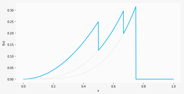
| "We can plot the resultant function for $x$ between 0 and 1, and we should recognise certain functions in segments of $x$. Starting with a quadratic curve from 0 to 1/2, we have a cubic curve from 1/2 to 2/3, a quartic from 2/3 to 3/4 and finally a flatline.\n", |
| "\n", |
| "\n", |
| "\n", |
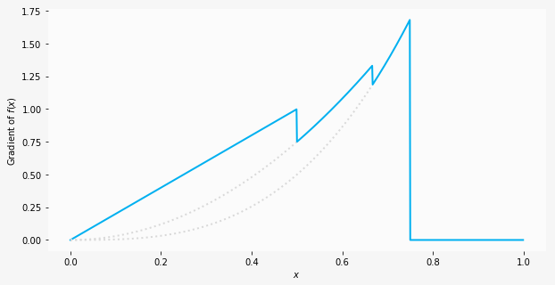
| "Using `autograd`, let's now find the gradient of this arbritrary function. We don't have a vectorized function in this case, because of the control flow, so let's also create a function to calculate the gradient using `autograd`." |
| ] |
| }, |
| { |
| "cell_type": "code", |
| "execution_count": 11, |
| "id": "9a7bd98b", |
| "metadata": {}, |
| "outputs": [ |
| { |
| "name": "stdout", |
| "output_type": "stream", |
| "text": [ |
| "[0.0, 0.20000000298023224, 0.4000000059604645, 0.6000000238418579, 0.800000011920929, 0.75, 1.0800000429153442, 1.371999979019165, 0.0, 0.0]\n" |
| ] |
| } |
| ], |
| "source": [ |
| "def get_grad(f, x):\n", |
| " x.attach_grad()\n", |
| " with autograd.record():\n", |
| " y = f(x)\n", |
| " y.backward()\n", |
| " return x.grad\n", |
| "\n", |
| "xs = mx.np.arange(0.0, 1.0, step=0.1)\n", |
| "grads = [get_grad(f, x).item() for x in xs]\n", |
| "print(grads)" |
| ] |
| }, |
| { |
| "cell_type": "markdown", |
| "id": "64ed59b8", |
| "metadata": {}, |
| "source": [ |
| "\n", |
| "\n", |
| "We can calculate the gradients by hand in this situation (since it's a toy example), and for the four segments discussed before we'd expect $2x$, $3x^2$, $4x^3$ and 0. As a spot check, for $x=0.6$ the hand calculated gradient would be $3x^2=1.08$, which equals `1.08` as computed by `autograd`.\n", |
| "\n", |
| "\n", |
| "## Advanced: Custom head gradients\n", |
| "\n", |
| "Most of the time `autograd` will be aware of the complete computational graph, and be able to calculate the gradients automatically. On a few rare occasions, you might have external post processing components (outside of MXNet Gluon) but still want to compute gradients with respect to MXNet Gluon network parameters.\n", |
| "\n", |
| "`autograd` enables this functionality by letting you pass in custom head gradients to `.backward()`. When nothing is specified (for the majority of cases), `autograd` will just used ones by default. Say we're interested in calculating $dz/dx$ but only calculate an intermediate variable $y$ using MXNet Gluon. We need to first calculate the head gradient $dz/dy$ (manually or otherwise), and then pass this to `.backward()`. `autograd` will then use this to calculate $dz/dx$, applying the chain rule.\n", |
| "\n", |
| "<p style=\"text-align:center\">\n", |
| " <video width=\"600\" controls playsinline autoplay muted loop>\n", |
| " <source src=\"/api/python/docs/_static/autograd_images/autograd_head_grad.mp4\" type=\"video/mp4\">\n", |
| " </video>\n", |
| "</p>\n", |
| "\n", |
| "As an example, let's take $y=x^3$ (calculated with `mxnet`) and $z=y^2$. (calculated with `numpy`). We can manually calculate $dz/dy=2y$ (once again with `numpy`), and use this as the head gradient for `autograd` to automatically calculate $dz/dx$. Applying the chain rule by hand we could calculate $dz/dx=6x^5$, so for $x=2$ we expect $dz/dx=192$. Let's check to see whether `autograd` calculates the same." |
| ] |
| }, |
| { |
| "cell_type": "code", |
| "execution_count": 12, |
| "id": "8ca5e8ab", |
| "metadata": {}, |
| "outputs": [ |
| { |
| "name": "stdout", |
| "output_type": "stream", |
| "text": [ |
| "[192.]\n" |
| ] |
| } |
| ], |
| "source": [ |
| "x = mx.np.array([2,])\n", |
| "x.attach_grad()\n", |
| "# compute y inside of mxnet (with `autograd`)\n", |
| "with autograd.record():\n", |
| " y = x**3\n", |
| "# compute dz/dy outside of mxnet\n", |
| "y_np = y.asnumpy()\n", |
| "z_np = y_np**2\n", |
| "dzdy_np = 2*y_np\n", |
| "# compute dz/dx inside of mxnet (given dz/dy)\n", |
| "dzdy = mx.np.array(dzdy_np)\n", |
| "y.backward(dzdy)\n", |
| "print(x.grad)" |
| ] |
| }, |
| { |
| "cell_type": "markdown", |
| "id": "73977513", |
| "metadata": {}, |
| "source": [ |
| "And as expected, we get a gradient of 192 for `x`." |
| ] |
| } |
| ], |
| "metadata": { |
| "language_info": { |
| "name": "python" |
| } |
| }, |
| "nbformat": 4, |
| "nbformat_minor": 5 |
| } |