TsFile Format

1. TsFile Design

This is an introduction to the design details of TsFile.

1.1 Variable Storage

Data Type Hardcode
- 0: BOOLEAN
- 1: INT32 (int)
- 2: INT64 (long)
- 3: FLOAT
- 4: DOUBLE
- 5: TEXT (String)
Encoding Type Hardcode
To improve the efficiency of data storage, it is necessary to encode data during data writing, thereby reducing the amount of disk space used. In the process of writing and reading data, the amount of data involved in the I/O operations can be reduced to improve performance. IoTDB supports the following encoding methods for different data types:
- 0: PLAIN
  - PLAIN encoding, the default encoding mode, i.e, no encoding, supports multiple data types. It has high compression and decompression efficiency while suffering from low space storage efficiency.
- 1: DICTIONARY
  - DICTIONARY encoding is lossless. It is suitable for TEXT data with low cardinality (i.e. low number of distinct values). It is not recommended to use it for high-cardinality data.
- 2: RLE
  - Run-length encoding is suitable for storing sequence with continuous integer values, and is not recommended for sequence data with most of the time different values.
  - Run-length encoding can also be used to encode floating-point numbers, while it is necessary to specify reserved decimal digits (MAX_POINT_NUMBER) when creating time series. It is more suitable to store sequence data where floating-point values appear continuously, monotonously increasing or decreasing, and it is not suitable for storing sequence data with high precision requirements after the decimal point or with large fluctuations.
    TS_2DIFF and RLE have precision limit for data type of float and double. By default, two decimal places are reserved. GORILLA is recommended.
- 3: DIFF
- 4: TS_2DIFF
  - Second-order differential encoding is more suitable for encoding monotonically increasing or decreasing sequence data, and is not recommended for sequence data with large fluctuations.
- 5: BITMAP
- 6: GORILLA_V1
  - GORILLA encoding is lossless. It is more suitable for numerical sequence with similar values and is not recommended for sequence data with large fluctuations.
  - Currently, there are two versions of GORILLA encoding implementation, it is recommended to use GORILLA instead of GORILLA_V1 (deprecated).
  - Usage restrictions: When using GORILLA to encode INT32 data, you need to ensure that there is no data point with the value Integer.MIN_VALUE in the sequence. When using GORILLA to encode INT64 data, you need to ensure that there is no data point with the value Long.MIN_VALUE in the sequence.
- 7: REGULAR
- 8: GORILLA

The correspondence between the data type and its supported encodings

Data Type	Supported Encoding
BOOLEAN	PLAIN, RLE
INT32	PLAIN, RLE, TS_2DIFF, GORILLA
INT64	PLAIN, RLE, TS_2DIFF, GORILLA
FLOAT	PLAIN, RLE, TS_2DIFF, GORILLA
DOUBLE	PLAIN, RLE, TS_2DIFF, GORILLA
TEXT	PLAIN, DICTIONARY

1.2 TsFile Overview

There are two parts in TsFile: Data Area and Index Area.

There are three concepts, from small to large, in Data Area:

Page: A page is a sequence of timeseries. It is the smallest unit in which a data block is deserialized.
Chunk: A chunk contains several pages in one timeseries. It is the smallest unit in which a data block is read by IO.
ChunkGroup: A chunk group contains several chunks in one entity.

There are three parts in Index Area:

TimeseriesIndex organized by timeseries, containing a header and list of ChunkIndex. The header records data type and statistics (maximum and minimum timestamps, etc.) of a time series in the file. The data block index list records the offsets of the chunks in the file, and the related statistics (maximum and minimum timestamps, etc.).
IndexOfTimeseriesIndex for index the offsets of TimeseriesIndex in the file.
BloomFilter for entities.

Here is the structure diagram of TsFile:

This TsFile contains two entities: d1, d2. Each entity contains three measurements: s1, s2, s3. 6 timeseries in total. Each timeseries contains 2 Chunks.

Query Process of reading d1.s1:

Deserialize IndexOfTimeseriesIndex, get the position of TimeseriesIndex of d1.s1
Deserialize and get the TimeseriesIndex of d1.s1
According to TimeseriesIndex of d1.s1, deserialize all ChunkIndex of d1.s1
According to each ChunkIndex of d1.s1, read its Chunk

1.2.1 Magic String and Version Number

A TsFile begins with a 6-byte magic string (TsFile) and a 6-byte version number (000002).

1.2.2 Data Area

ChunkGroup

A ChunkGroup stores the data of an entity for a period of time. It consists of several Chunk, a byte delimiter0x00 and a ChunkFooter.

Chunk

A Chunk stores the data of a measurement for a period of time. The data in a chunk is stored in time increment order. It consists of a byte 0x01 as the marker, following a ChunkHeader and an array of Page.

ChunkHeader

Member	Type	Description
measurementID	String	Name of measurement
dataSize	int	Size of this chunk
dataType	TSDataType	Data type of this chuck
compressionType	CompressionType	Compression Type
encodingType	TSEncoding	Encoding Type
numOfPages	int	Number of pages

Page

A Page stores a sequence of timeseries. It is the smallest unit in which a data block is deserialized. It contains a PageHeader and the actual data (encoded time-value pairs).

PageHeader Structure:

Member	Type	Description
uncompressedSize	int	Data size before compressing
compressedSize	int	Data size after compressing(if use SNAPPY)
statistics	Statistics	Statistics values

Here is the detailed information for statistics:

Member	Description	DoubleStatistics	FloatStatistics	IntegerStatistics	LongStatistics	BinaryStatistics	BooleanStatistics
count	number of time-value points	long	long	long	long	long	long
startTime	start time	long	long	long	long	long	long
endTime	end time	long	long	long	long	long	long
minValue	min value	double	float	int	long	-	-
maxValue	max value	double	float	int	long	-	-
firstValue	first value	double	float	int	long	Binary	boolean
lastValue	last value	double	float	int	long	Binary	boolean
sumValue	sum value	double	double	double	double	-	-

ChunkGroupFooter

Member	Type	Description
entityID	String	Name of entity
dataSize	long	Data size of the ChunkGroup
numberOfChunks	int	Number of chunks

1.2.3 Index Area

1.2.3.1 ChunkIndex

The first part of index is ChunkIndex :

Member	Type	Description
measurementUid	String	Name of measurement
offsetOfChunkHeader	long	Start offset of ChunkHeader
tsDataType	TSDataType	Data type
statistics	Statistics	Statistic values

1.2.3.2 TimeseriesIndex

The second part of index is TimeseriesIndex:

Member	Type	Description
measurementUid	String	Name of measurement
tsDataType	short	Data type
startOffsetOfChunkIndexList	long	Start offset of ChunkIndex list
ChunkIndexListDataSize	int	ChunkIndex list size
statistics	Statistics	Statistic values

1.2.3.3 IndexOfTimeseriesIndex (Secondary Index)

The third part of index is IndexOfTimeseriesIndex:

Member	Type	Description
IndexTree	IndexNode	Root index node of IndexTree
offsetOfIndexArea	long	offset of index area
bloomFilter	BloomFilter	bloom filter

IndexNode has members as below:

Member	Type	Description
children	List	IndexEntry list
endOffset	long	EndOffset of this IndexNode
nodeType	IndexNodeType	IndexNode type

IndexEntry has members as below:

Member	Type	Description
name	String	Name of related entity or measurement
offset	long	offset

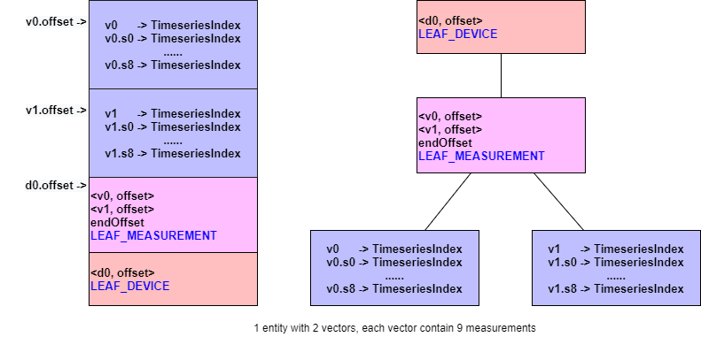
All IndexNode forms an index tree (secondary index) like a B+ tree, which consists of two levels: entity index level and measurement index level. The IndexNodeType has four enums: INTERNAL_ENTITY, LEAF_ENTITY, INTERNAL_MEASUREMENT, LEAF_MEASUREMENT, which indicates the internal or leaf node of entity index level and measurement index level respectively. Only the LEAF_MEASUREMENT nodes point to TimeseriesIndex.

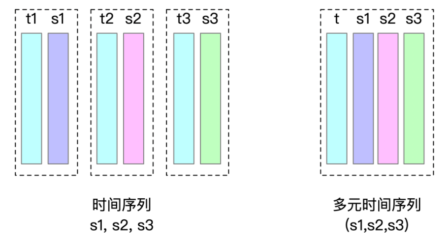
Consider the introduction of multi-variable timeseries, each multi-variable timeseries is called a vector with a TimeColumn. For example, the multi-variable timeseries vector1 belongs to the entity d , with two measurements s1, s2. i.e. d1.vector1.(s1,s2), we call vector1 as TimeColumn. In the storage, you need to store an extra Chunk of vector1.

Except for TimeColumn, measurements of a multi-variable timeseries are concatenated with TimeColumn when constructing IndexOfTimeseriesIndex, e.g. we Indicates vector1.s1 as a measurement.

From v0.13, IoTDB supports Multi-variable Timeseries. A multi-variable measurements of an entity corresponds to a multi-variable timeseries. These timeseries are called multi-variable timeseries, also called aligned timeseries.
Multi-variable timeseries need to be created, inserted and deleted at the same time. However, when querying, you can query each sub-measurement separately.
By using multi-variable timeseries, the timestamp columns of a group of multi-variable timeseries need to be stored only once in memory and disk when inserting data, instead of once per timeseries.

Here are seven detailed examples.

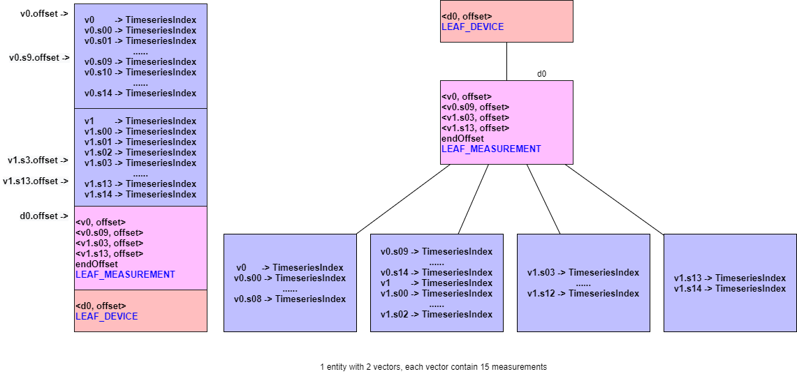
The degree of the index tree (that is, the max number of each node's children) could be configured by users, and is 256 by default. In the examples below, we assume max_degree_of_index_node = 10.

Note that the keys are arranged in dictionary order in each type of nodes (ENTITY, MEASUREMENT) of the index tree. In the following example, we assumed that the dictionary order di<dj if i<j. (Otherwise, in fact, the dictionary order of [d1,d2,... .d10] should be [d1,d10,d2,.... .d9])

Example 1~4 is an example of a single-variable timeseries.

Example 5~6 is an example of a multi-variale timeseries. Example 7 is a comprehensive example.

Example 1: 5 entities with 5 measurements each
Example 2: 1 entity with 150 measurements

In the case of 1 entity with 150 measurements: The number of measurements exceeds max_degree_of_index_node, so the tree has only measurement index level by default. In this level, each IndexNode is composed of no more than 10 index entries. The nodes that point to TimeseriesIndex directly are LEAF_MEASUREMENT type. Other nodes are not leaf nodes of measurement index level, so they are INTERNAL_MEASUREMENT type. The root node is INTERNAL_ENTITY type.

Example 3: 150 entities with 1 measurement each

In the case of 150 entities with 1 measurement each: The number of entities exceeds max_degree_of_index_node, so the entity index level and measurement index level of the tree are both formed. In these two levels, each IndexNode is composed of no more than 10 index entries. The nodes that point to TimeseriesIndex directly are LEAF_MEASUREMENT type. The root nodes of measurement index level are also the leaf nodes of entity index level, which are LEAF_ENTITY type. Other nodes and root node of index tree are not leaf nodes of entity level, so they are INTERNAL_ENTITY type.

Example 4: 150 entities with 150 measurements each

In the case of 150 entities with 150 measurements each: The numbers of entities and measurements both exceed max_degree_of_index_node, so the entity index level and measurement index level are both formed. In these two levels, each IndexNode is composed of no more than 10 index entries. As is described before, from the root node to the leaf nodes of entity index level, their types are INTERNAL_ENTITY and LEAF_ENTITY; each leaf node of entity index level can be seen as the root node of measurement index level, and from here to the leaf nodes of measurement index level, their types are INTERNAL_MEASUREMENT and LEAF_MEASUREMENT.

Example 5: 1 entities with 2 vectors, 9 measurements for each vector
Example 6: 1 entities with 2 vectors, 15 measurements for each vector

Example 7: 2 entities, measurements of entities are shown in the following table

entity: d0	entity: d1
【Single-variable Tmeseries】s0,s1...,s4	【Single-variable Tmeseries】s0,s1,...s14
【Multi-variable Timeseries】v0.(s5,s6,...,s14)	【Multi-variable Timeseries】v0.(s15,s16,..s18)
【Single-variable Tmeseries】z15,z16,..,z18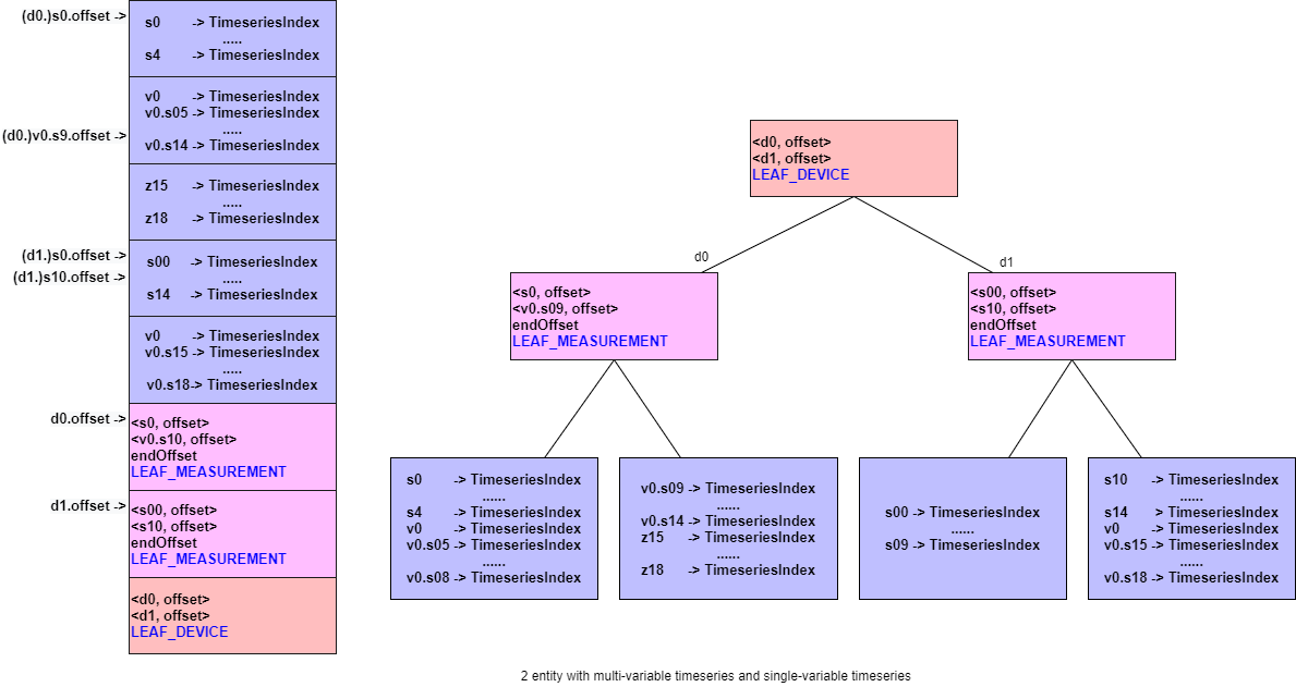

The IndexTree is designed as tree structure so that not all the TimeseriesIndex need to be read when the number of entities or measurements is too large. Only reading specific IndexTree nodes according to requirement and reducing I/O could speed up the query. More reading process of TsFile in details will be described in the last section of this chapter.

1.2.4 Magic String

A TsFile ends with a 6-byte magic string (TsFile).

Congratulations! You have finished the journey of discovering TsFile.

2. A TsFile Visualization Example

v0.8

v0.9 / 000001

v0.10 / 000002

v0.12 / 000003

3. TsFile Tool Set

3.1 IoTDB Data Directory Overview Tool

After building the server, the startup script of this tool will appear under the server\target\iotdb-server-{version}\tools\tsfileToolSet directory.

Command:

For Windows:

.\print-iotdb-data-dir.bat <path of your IoTDB data directory or directories separated by comma> (<path of the file for saving the output result>)

For Linux or MacOs:

./print-iotdb-data-dir.sh <path of your IoTDB data directory or directories separated by comma> (<path of the file for saving the output result>)

An example on Windows:

D:\iotdb\server\target\iotdb-server-{version}\tools\tsfileToolSet>.\print-iotdb-data-dir.bat D:\\data\data
|````````````````````````
Starting Printing the IoTDB Data Directory Overview
|````````````````````````
output save path:IoTDB_data_dir_overview.txt
TsFile data dir num:1
21:17:38.841 [main] WARN org.apache.iotdb.tsfile.common.conf.TSFileDescriptor - Failed to find config file iotdb-engine.properties at classpath, use default configuration
|==============================================================
|D:\\data\data
|--sequence
|  |--root.ln.wf01.wt01
|  |  |--1575813520203-101-0.tsfile
|  |  |--1575813520203-101-0.tsfile.resource
|  |  |  |--device root.ln.wf01.wt01, start time 1 (1970-01-01T08:00:00.001+08:00[GMT+08:00]), end time 5 (1970-01-01T08:00:00.005+08:00[GMT+08:00])
|  |  |--1575813520669-103-0.tsfile
|  |  |--1575813520669-103-0.tsfile.resource
|  |  |  |--device root.ln.wf01.wt01, start time 100 (1970-01-01T08:00:00.100+08:00[GMT+08:00]), end time 300 (1970-01-01T08:00:00.300+08:00[GMT+08:00])
|  |  |--1575813521372-107-0.tsfile
|  |  |--1575813521372-107-0.tsfile.resource
|  |  |  |--device root.ln.wf01.wt01, start time 500 (1970-01-01T08:00:00.500+08:00[GMT+08:00]), end time 540 (1970-01-01T08:00:00.540+08:00[GMT+08:00])
|--unsequence
|  |--root.ln.wf01.wt01
|  |  |--1575813521063-105-0.tsfile
|  |  |--1575813521063-105-0.tsfile.resource
|  |  |  |--device root.ln.wf01.wt01, start time 10 (1970-01-01T08:00:00.010+08:00[GMT+08:00]), end time 50 (1970-01-01T08:00:00.050+08:00[GMT+08:00])
|==============================================================

3.2 TsFileResource Print Tool

After building the server, the startup script of this tool will appear under the server\target\iotdb-server-{version}\tools\tsfileToolSet directory.

Command:

For Windows:

.\print-tsfile-resource-files.bat <path of your TsFileResource directory>

For Linux or MacOs:

./print-tsfile-resource-files.sh <path of your TsFileResource directory>

An example on Windows:

D:\iotdb\server\target\iotdb-server-{version}\tools\tsfileToolSet>.\print-tsfile-resource-files.bat D:\data\data\sequence\root.vehicle
|````````````````````````
Starting Printing the TsFileResources
|````````````````````````
12:31:59.861 [main] WARN org.apache.iotdb.db.conf.IoTDBDescriptor - Cannot find IOTDB_HOME or IOTDB_CONF environment variable when loading config file iotdb-engine.properties, use default configuration
analyzing D:\data\data\sequence\root.vehicle\1572496142067-101-0.tsfile ...
device root.vehicle.d0, start time 3000 (1970-01-01T08:00:03+08:00[GMT+08:00]), end time 100999 (1970-01-01T08:01:40.999+08:00[GMT+08:00])
analyzing the resource file finished.

3.3 TsFile Sketch Tool

After building the server, the startup script of this tool will appear under the server\target\iotdb-server-{version}\tools\tsfileToolSet directory.

Command:

For Windows:

.\print-tsfile-sketch.bat <path of your TsFile> (<path of the file for saving the output result>)

Note that if <path of the file for saving the output result> is not set, the default path “TsFile_sketch_view.txt” will be used.

For Linux or MacOs:

./print-tsfile-sketch.sh <path of your TsFile> (<path of the file for saving the output result>)

Note that if <path of the file for saving the output result> is not set, the default path “TsFile_sketch_view.txt” will be used.

An example on macOS:

/iotdb/server/target/iotdb-server-{version}/tools/tsfileToolSet$ ./print-tsfile-sketch.sh test.tsfile
｜````````````````````````
Starting Printing the TsFile Sketch
｜````````````````````````
TsFile path:test.tsfile
Sketch save path:TsFile_sketch_view.txt
-------------------------------- TsFile Sketch --------------------------------
file path: test.tsfile
file length: 15462
14:40:55.619 [main] INFO org.apache.iotdb.tsfile.read.TsFileSequenceReader - Start reading file test.tsfile metadata from 15356, length 96

            POSITION|	CONTENT
            -------- 	-------
                   0|	[magic head] TsFile
                   6|	[version number] 3
|||||||||||||||||||||	[Chunk Group] of root.sg_1.d1, num of Chunks:4
                   7|	[Chunk Group Header]
                    |		[marker] 0
                    |		[deviceID] root.sg_1.d1
                  21|	[Chunk] of s6, numOfPoints:1000, time range:[0,999], tsDataType:INT64, 
                     	startTime: 0 endTime: 999 count: 1000 [minValue:6,maxValue:9996,firstValue:6,lastValue:9996,sumValue:5001000.0]
                    |		[chunk header] marker=5, measurementId=s6, dataSize=1826, serializedSize=9
                    |		[chunk] java.nio.HeapByteBuffer[pos=0 lim=1826 cap=1826]
                    |		[page]  CompressedSize:1822, UncompressedSize:1951
                1856|	[Chunk] of s4, numOfPoints:1000, time range:[0,999], tsDataType:INT64, 
                     	startTime: 0 endTime: 999 count: 1000 [minValue:4,maxValue:9994,firstValue:4,lastValue:9994,sumValue:4999000.0]
                    |		[chunk header] marker=5, measurementId=s4, dataSize=1826, serializedSize=9
                    |		[chunk] java.nio.HeapByteBuffer[pos=0 lim=1826 cap=1826]
                    |		[page]  CompressedSize:1822, UncompressedSize:1951
                3691|	[Chunk] of s2, numOfPoints:1000, time range:[0,999], tsDataType:INT64, 
                     	startTime: 0 endTime: 999 count: 1000 [minValue:3,maxValue:9993,firstValue:3,lastValue:9993,sumValue:4998000.0]
                    |		[chunk header] marker=5, measurementId=s2, dataSize=1826, serializedSize=9
                    |		[chunk] java.nio.HeapByteBuffer[pos=0 lim=1826 cap=1826]
                    |		[page]  CompressedSize:1822, UncompressedSize:1951
                5526|	[Chunk] of s5, numOfPoints:1000, time range:[0,999], tsDataType:INT64, 
                     	startTime: 0 endTime: 999 count: 1000 [minValue:5,maxValue:9995,firstValue:5,lastValue:9995,sumValue:5000000.0]
                    |		[chunk header] marker=5, measurementId=s5, dataSize=1826, serializedSize=9
                    |		[chunk] java.nio.HeapByteBuffer[pos=0 lim=1826 cap=1826]
                    |		[page]  CompressedSize:1822, UncompressedSize:1951
|||||||||||||||||||||	[Chunk Group] of root.sg_1.d1 ends
|||||||||||||||||||||	[Chunk Group] of root.sg_1.d2, num of Chunks:4
                7361|	[Chunk Group Header]
                    |		[marker] 0
                    |		[deviceID] root.sg_1.d2
                7375|	[Chunk] of s2, numOfPoints:1000, time range:[0,999], tsDataType:INT64, 
                     	startTime: 0 endTime: 999 count: 1000 [minValue:3,maxValue:9993,firstValue:3,lastValue:9993,sumValue:4998000.0]
                    |		[chunk header] marker=5, measurementId=s2, dataSize=1826, serializedSize=9
                    |		[chunk] java.nio.HeapByteBuffer[pos=0 lim=1826 cap=1826]
                    |		[page]  CompressedSize:1822, UncompressedSize:1951
                9210|	[Chunk] of s4, numOfPoints:1000, time range:[0,999], tsDataType:INT64, 
                     	startTime: 0 endTime: 999 count: 1000 [minValue:4,maxValue:9994,firstValue:4,lastValue:9994,sumValue:4999000.0]
                    |		[chunk header] marker=5, measurementId=s4, dataSize=1826, serializedSize=9
                    |		[chunk] java.nio.HeapByteBuffer[pos=0 lim=1826 cap=1826]
                    |		[page]  CompressedSize:1822, UncompressedSize:1951
               11045|	[Chunk] of s6, numOfPoints:1000, time range:[0,999], tsDataType:INT64, 
                     	startTime: 0 endTime: 999 count: 1000 [minValue:6,maxValue:9996,firstValue:6,lastValue:9996,sumValue:5001000.0]
                    |		[chunk header] marker=5, measurementId=s6, dataSize=1826, serializedSize=9
                    |		[chunk] java.nio.HeapByteBuffer[pos=0 lim=1826 cap=1826]
                    |		[page]  CompressedSize:1822, UncompressedSize:1951
               12880|	[Chunk] of s5, numOfPoints:1000, time range:[0,999], tsDataType:INT64, 
                     	startTime: 0 endTime: 999 count: 1000 [minValue:5,maxValue:9995,firstValue:5,lastValue:9995,sumValue:5000000.0]
                    |		[chunk header] marker=5, measurementId=s5, dataSize=1826, serializedSize=9
                    |		[chunk] java.nio.HeapByteBuffer[pos=0 lim=1826 cap=1826]
                    |		[page]  CompressedSize:1822, UncompressedSize:1951
|||||||||||||||||||||	[Chunk Group] of root.sg_1.d2 ends
               14715|	[marker] 2
               14716|	[TimeseriesIndex] of root.sg_1.d1.s2, tsDataType:INT64
                    |		[ChunkIndex] s2, offset=3691
                    |		[startTime: 0 endTime: 999 count: 1000 [minValue:3,maxValue:9993,firstValue:3,lastValue:9993,sumValue:4998000.0]] 
               14788|	[TimeseriesIndex] of root.sg_1.d1.s4, tsDataType:INT64
                    |		[ChunkIndex] s4, offset=1856
                    |		[startTime: 0 endTime: 999 count: 1000 [minValue:4,maxValue:9994,firstValue:4,lastValue:9994,sumValue:4999000.0]] 
               14860|	[TimeseriesIndex] of root.sg_1.d1.s5, tsDataType:INT64
                    |		[ChunkIndex] s5, offset=5526
                    |		[startTime: 0 endTime: 999 count: 1000 [minValue:5,maxValue:9995,firstValue:5,lastValue:9995,sumValue:5000000.0]] 
               14932|	[TimeseriesIndex] of root.sg_1.d1.s6, tsDataType:INT64
                    |		[ChunkIndex] s6, offset=21
                    |		[startTime: 0 endTime: 999 count: 1000 [minValue:6,maxValue:9996,firstValue:6,lastValue:9996,sumValue:5001000.0]] 
               15004|	[TimeseriesIndex] of root.sg_1.d2.s2, tsDataType:INT64
                    |		[ChunkIndex] s2, offset=7375
                    |		[startTime: 0 endTime: 999 count: 1000 [minValue:3,maxValue:9993,firstValue:3,lastValue:9993,sumValue:4998000.0]] 
               15076|	[TimeseriesIndex] of root.sg_1.d2.s4, tsDataType:INT64
                    |		[ChunkIndex] s4, offset=9210
                    |		[startTime: 0 endTime: 999 count: 1000 [minValue:4,maxValue:9994,firstValue:4,lastValue:9994,sumValue:4999000.0]] 
               15148|	[TimeseriesIndex] of root.sg_1.d2.s5, tsDataType:INT64
                    |		[ChunkIndex] s5, offset=12880
                    |		[startTime: 0 endTime: 999 count: 1000 [minValue:5,maxValue:9995,firstValue:5,lastValue:9995,sumValue:5000000.0]] 
               15220|	[TimeseriesIndex] of root.sg_1.d2.s6, tsDataType:INT64
                    |		[ChunkIndex] s6, offset=11045
                    |		[startTime: 0 endTime: 999 count: 1000 [minValue:6,maxValue:9996,firstValue:6,lastValue:9996,sumValue:5001000.0]] 
|||||||||||||||||||||
               15292|	[IndexOfTimerseriesIndex Node] type=LEAF_MEASUREMENT
                    |		<s2, 14716>
                    |		<s6, 14932>
                    |		<endOffset, 15004>
               15324|	[IndexOfTimerseriesIndex Node] type=LEAF_MEASUREMENT
                    |		<s2, 15004>
                    |		<s6, 15220>
                    |		<endOffset, 15292>
               15356|	[TsFileMetadata]
                    |		[meta offset] 14715
                    |		[num of devices] 2
                    |		2 key&TsMetadataIndex
                    |		[bloom filter bit vector byte array length] 32
                    |		[bloom filter bit vector byte array] 
                    |		[bloom filter number of bits] 256
                    |		[bloom filter number of hash functions] 5
               15452|	[TsFileMetadataSize] 96
               15456|	[magic tail] TsFile
               15462|	END of TsFile
---------------------------- IndexOfTimerseriesIndex Tree -----------------------------
	[MetadataIndex:LEAF_DEVICE]
	└───[root.sg_1.d1,15292]
			[MetadataIndex:LEAF_MEASUREMENT]
			└───[s2,14716]
			└───[s6,14932]
	└───[root.sg_1.d2,15324]
			[MetadataIndex:LEAF_MEASUREMENT]
			└───[s2,15004]
			└───[s6,15220]]
---------------------------------- TsFile Sketch End ----------------------------------

3.4 TsFileSequenceRead

You can also use example/tsfile/org/apache/iotdb/tsfile/TsFileSequenceRead to sequentially print a TsFile's content.

3.5 Vis Tool

Vis is a tool that visualizes the time layouts and cout aggregation of chunk data in TsFiles. You can use this tool to facilitate debugging, check the distribution of data, etc. Please feel free to play around with it, and let us know your thoughts.

A single long narrow rectangle in the figure shows the visdata of a single chunk in a TsFile. Visdata contains [tsName, fileName, chunkId, startTime, endTime, pointCountNum].
The position of a rectangle on the x-axis is defined by the startTime and endTime of the chunk data.
The position of a rectangle on the y-axis is defined simultaneously by
- (a)showSpecific: the specific set of time series to be plotted;
- (b) seqKey/unseqKey display policies: extract seqKey or unseqKey from statisfied keys under different display policies:
  - b-1) unseqKey identifies tsName and fileName, so chunk data with the same fileName and tsName but different chunkIds are plotted on the same line.
  - b-2) seqKey identifies tsName, so chunk data with the same tsName but different fileNames and chunkIds are plotted on the same line;
- (c)isFileOrder: sort seqKey&unseqKey according to isFileOrder, true to sort seqKeys&unseqKeys by fileName priority, false to sort seqKeys&unseqKeys by tsName priority. When multiple time series are displayed on a graph at the same time, this parameter can provide users with these two observation perspectives.

3.5.1 How to run Vis

The source code contains two files: TsFileExtractVisdata.java and vis.m. TsFileExtractVisdata.java extracts, from input tsfiles, necessary visualization information, which is what vis.m needs to plot figures.

Simply put, you first run TsFileExtractVisdata.java and then run vis.m.

Step 1: run TsFileExtractVisdata.java

TsFileExtractVisdata.java extracts visdata [tsName, fileName, chunkId, startTime, endTime, pointCountNum] from every chunk of the input TsFiles and write them to the specified output path.

After building the server, the startup script of this tool will appear under the server\target\iotdb-server-{version}\tools\tsfileToolSet directory.

Command:

For Windows:

.\print-tsfile-visdata.bat path1 seqIndicator1 path2 seqIndicator2 ... pathN seqIndicatorN outputPath

For Linux or MacOs:

./print-tsfile-visdata.sh path1 seqIndicator1 path2 seqIndicator2 ... pathN seqIndicatorN outputPath

Args: [path1 seqIndicator1 path2 seqIndicator2 ... pathN seqIndicatorN outputPath]

Details:

2N+1 args in total.
seqIndicator should be ‘true’ or ‘false’ (not case sensitive). ‘true’ means is the file is sequence, ‘false’ means the file is unsequence.
Path can be the full path of a tsfile or a directory path. If it is a directory path, make sure that all tsfiles in this directory have the same seqIndicator.
The input TsFiles should all be sealed. The handle of unsealed TsFile is left as future work when in need.

Step 2: run vis.m

vis.m load visdata generated by TsFileExtractVisdata, and then plot figures given the loaded visdata and two plot parameters: showSpecific and isFileOrder.

function [timeMap,countMap] = loadVisData(filePath,timestampUnit)
% Load visdata generated by TsFileExtractVisdata.
%
% filePath: the path of visdata.
% The format is [tsName,fileName,chunkId,startTime,endTime,pointCountNum].
% `tsName` and `fileName` are string, the others are long value.
% If the tsfile is unsequence file, `fileName` will contain "unseq" as an
% indicator, which is guaranteed by TsFileExtractVisdata.
%
% timestampUnit(not case sensitive):
%   'us' if the timestamp is microsecond, e.g., 1621993620816000
%   'ms' if it is millisecond, e.g., 1621993620816
%   's' if it is second, e.g., 1621993620
%
% timeMap: record the time range of every chunk.
% Key [tsName][fileName][chunkId] identifies the only chunk. Value is
% [startTime,endTime] of the chunk.
%
% countMap: record the point count number of every chunk. Key is the same
% as that of timeMap. Value is pointCountNum.

function draw(timeMap,countMap,showSpecific,isFileOrder)
% Plot figures given the loaded data and two plot parameters:
% `showSpecific` and `isFileOrder`.
%
% process: 1) traverse `keys(timeMap)` to get the position arrangements on
%          the y axis dynamically, which is defined simultaneously by
%           (a)`showSpecific`: traverse `keys(timeMap)`, filter out keys
%          that don't statisfy `showSpecific`.
%           (b) seqKey/unseqKey display policies: extract seqKey or unseqKey
%          from statisfied keys under different display policies:
%               b-1) unseqKey identifies tsName and fileName, so chunk data with the
%               same fileName and tsName but different chunkIds are
%               plotted on the same line.
%               b-2) seqKey identifies tsName, so chunk data with the same tsName but
%               different fileNames and chunkIds are plotted on the same
%               line.
%           (c)`isFileOrder`: sort seqKey&unseqKey according to `isFileOrder`,
%          finally get the position arrangements on the y axis.
%          2) traverse `keys(timeMap)` again, get startTime&endTime from
%          `treeMap` as positions on the x axis, combined with the
%          positions on the y axis from the last step, finish plot.
%
% timeMap,countMap: generated by loadVisData function.
%
% showSpecific: the specific set of time series to be plotted.
%               If showSpecific is empty{}, then all loaded time series
%               will be plotted.
%               Note: Wildcard matching is not supported now. In other
%               words, showSpecific only support full time series path
%               names.
%
% isFileOrder: true to sort seqKeys&unseqKeys by fileName priority, false
%              to sort seqKeys&unseqKeys by tsName priority.

3.5.2 Examples

Example 1

Use the tsfiles written by IoTDBLargeDataIT.insertData with a little modification: add statement.execute("flush"); at the end of IoTDBLargeDataIT.insertData.

Step 1: run TsFileExtractVisdata.java

.\print-tsfile-visdata.bat data\sequence true data\unsequence false D:\visdata1.csv

or equivalently:

.\print-tsfile-visdata.bat data\sequence\root.vehicle\0\0\1622743492580-1-0.tsfile true data\sequence\root.vehicle\0\0\1622743505092-2-0.tsfile true data\sequence\root.vehicle\0\0\1622743505573-3-0.tsfile true data\unsequence\root.vehicle\0\0\1622743505901-4-0.tsfile false D:\visdata1.csv

Step 2: run vis.m

clear all;close all;

% 1. load visdata generated by TsFileExtractVisdata
filePath = 'D:\visdata1.csv';
[timeMap,countMap] = loadVisData(filePath,'ms'); % mind the timestamp unit

% 2. plot figures given the loaded data and two plot parameters:
% `showSpecific` and `isFileOrder`
draw(timeMap,countMap,{},false)
title("draw(timeMap,countMap,\{\},false)")

draw(timeMap,countMap,{},true)
title("draw(timeMap,countMap,\{\},true)")

draw(timeMap,countMap,{'root.vehicle.d0.s0'},false)
title("draw(timeMap,countMap,{'root.vehicle.d0.s0'},false)")

draw(timeMap,countMap,{'root.vehicle.d0.s0','root.vehicle.d0.s1'},false)
title("draw(timeMap,countMap,{'root.vehicle.d0.s0','root.vehicle.d0.s1'},false)")

draw(timeMap,countMap,{'root.vehicle.d0.s0','root.vehicle.d0.s1'},true)
title("draw(timeMap,countMap,{'root.vehicle.d0.s0','root.vehicle.d0.s1'},true)")

Plot results:

Appendix

Big Endian
- For Example, the int 0x8 will be stored as 00 00 00 08, replace by 08 00 00 00
String with Variable Length
- The format is int size plus String literal. Size can be zero.
- Size equals the number of bytes this string will take, and it may not equal to the length of the string.
- For example “sensor_1” will be stored as 00 00 00 08 plus the encoding(ASCII) of “sensor_1”.
- Note that for the file signature “TsFile000001” (MAGIC STRING + Version Number), the size(12) and encoding(ASCII) is fixed so there is no need to put the size before this string literal.
Compressing Type Hardcode
- 0: UNCOMPRESSED
- 1: SNAPPY
- 2: GZIP
- 3: LZO
- 4: SDT
- 5: PAA
- 6: PLA
- 7: LZ4