[docs](images) Update Partial Optimized Images (#683)
diff --git a/docs/admin-manual/cluster-management/load-balancing.md b/docs/admin-manual/cluster-management/load-balancing.md
index a904c1d..9e1553d 100644
--- a/docs/admin-manual/cluster-management/load-balancing.md
+++ b/docs/admin-manual/cluster-management/load-balancing.md
@@ -514,22 +514,22 @@
 Then add the following in it

 ```bash
-events {
-worker_connections 1024;
-}
-stream {
-  upstream mysqld {
-      hash $remote_addr consistent;
-      server 172.31.7.119:9030 weight=1 max_fails=2 fail_timeout=60s;
-      ##注意这里如果是多个FE,加载这里就行了
-  }
-  ###这里是配置代理的端口,超时时间等
-  server {
-      listen 6030;
-      proxy_connect_timeout 300s;
-      proxy_timeout 300s;
-      proxy_pass mysqld;
-  }
+events {
+worker_connections 1024;
+}
+stream {
+  upstream mysqld {
+      hash $remote_addr consistent;
+      server 172.31.7.119:9030 weight=1 max_fails=2 fail_timeout=60s;
+      ## Note: If there are multiple FEs, just load them here.
+  }
+  ### Configuration for proxy port, timeout, etc.
+  server {
+      listen 6030;
+      proxy_connect_timeout 300s;
+      proxy_timeout 300s;
+      proxy_pass mysqld;
+  }
 }
 ```
diff --git a/docs/admin-manual/fe/node-action.md b/docs/admin-manual/fe/node-action.md
index 842d58c..70dd50f 100644
--- a/docs/admin-manual/fe/node-action.md
+++ b/docs/admin-manual/fe/node-action.md
@@ -24,7 +24,7 @@
 under the License.
 -->

-# Node Action
+

 ## Request

@@ -220,7 +220,8 @@

 ### Response
 `GET /rest/v2/manager/node/configuration_name`
-```
+
+```json
 {
     "msg": "success",
     "code": 0,
@@ -237,7 +238,8 @@
 ```

 `GET /rest/v2/manager/node/node_list`
-```
+
+```json
 {
     "msg": "success",
     "code": 0,
@@ -254,27 +256,28 @@
 ```

 `POST /rest/v2/manager/node/configuration_info?type=fe`
-```
-{
-    "msg": "success",
-    "code": 0,
-    "data": {
-        "column_names": [
-            "配置项",
-            "节点",
-            "节点类型",
-            "配置值类型",
-            "MasterOnly",
-            "配置值",
-            "可修改"
-        ],
-        "rows": [
-            [
-                ""
-            ]
-        ]
-    },
-    "count": 0
+
+```json
+{
+    "msg": "success",
+    "code": 0,
+    "data": {
+        "column_names": [
+            "Configuration Item",
+            "Node",
+            "Node Type",
+            "Configuration Value Type",
+            "MasterOnly",
+            "Configuration Value",
+            "Modifiable"
+        ],
+        "rows": [
+            [
+                ""
+            ]
+        ]
+    },
+    "count": 0
 }
 ```

@@ -285,12 +288,12 @@
     "code": 0,
     "data": {
         "column_names": [
-            "配置项",
-            "节点",
-            "节点类型",
-            "配置值类型",
-            "配置值",
-            "可修改"
+            "Configuration Item",
+            "Node",
+            "Node Type",
+            "Configuration Value Type",
+            "Configuration Value",
+            "Modifiable"
         ],
         "rows": [
             [
@@ -308,7 +311,8 @@

     POST /rest/v2/manager/node/configuration_info?type=fe
     body:
-    ```
+
+    ```json
     {
         "conf_name":[
             "agent_task_resend_wait_time_ms"
@@ -317,33 +321,34 @@
     ```

     Response:
-    ```
-    {
-        "msg": "success",
-        "code": 0,
-        "data": {
-            "column_names": [
-                "配置项",
-                "节点",
-                "节点类型",
-                "配置值类型",
-                "MasterOnly",
-                "配置值",
-                "可修改"
-            ],
-            "rows": [
-                [
-                    "agent_task_resend_wait_time_ms",
-                    "127.0.0.1:8030",
-                    "FE",
-                    "long",
-                    "true",
-                    "50000",
-                    "true"
-                ]
-            ]
-        },
-        "count": 0
+
+    ```json
+    {
+    "msg": "success",
+    "code": 0,
+    "data": {
+        "column_names": [
+            "Configuration Item",
+            "Node",
+            "Node Type",
+            "Configuration Value Type",
+            "MasterOnly",
+            "Configuration Value",
+            "Modifiable"
+        ],
+        "rows": [
+            [
+                "agent_task_resend_wait_time_ms",
+                "127.0.0.1:8030",
+                "FE",
+                "long",
+                "true",
+                "50000",
+                "true"
+            ]
+        ]
+    },
+    "count": 0
     }
     ```

@@ -358,7 +363,8 @@
 Used to modify fe or be node configuration values

 ### Request body
-```
+
+```json
 {
 	"config_name":{
 		"node":[
@@ -377,7 +383,8 @@

 ### Response
 `GET /rest/v2/manager/node/configuration_name`
-```
+
+``` json
 {
 	"msg": "",
 	"code": 0,
@@ -403,7 +410,8 @@

     POST /rest/v2/manager/node/set_config/fe
     body:
-    ```
+
+    ```json
     {
         "agent_task_resend_wait_time_ms":{
             "node":[
@@ -454,7 +462,8 @@
 action:ADD/DROP/DECOMMISSION

 ### Request body
-```
+
+```json
 {
     "hostPorts": ["127.0.0.1:9050"],
     "properties": {
@@ -467,7 +476,8 @@
 ```

 ### Response
-```
+
+```json
 {
     "msg": "Error",
     "code": 1,
@@ -486,14 +496,16 @@

    post /rest/v2/manager/node/ADD/be
    Request body
-    ```
+
+    ```json
     {
         "hostPorts": ["127.0.0.1:9050"]
     }
     ```

    Response
-    ```
+
+    ```json
     {
         "msg": "success",
         "code": 0,
@@ -506,14 +518,16 @@

    post /rest/v2/manager/node/DROP/be
    Request body
-    ```
+
+    ```json
     {
         "hostPorts": ["127.0.0.1:9050"]
     }
     ```

    Response
-    ```
+
+    ```json
     {
         "msg": "success",
         "code": 0,
@@ -526,14 +540,14 @@

    post /rest/v2/manager/node/DECOMMISSION/be
    Request body
-    ```
+    ```json
     {
         "hostPorts": ["127.0.0.1:9050"]
     }
     ```

    Response
-    ```
+    ```json
     {
         "msg": "success",
         "code": 0,
@@ -553,7 +567,7 @@
 action:ADD/DROP

 ### Request body
-```
+```json
 {
     "role": "FOLLOWER",
     "hostPort": "127.0.0.1:9030"
@@ -564,7 +578,7 @@
 ```

 ### Response
-```
+```json
 {
     "msg": "Error",
     "code": 1,
@@ -583,7 +597,7 @@

    post /rest/v2/manager/node/ADD/fe
    Request body
-    ```
+    ```json
     {
         "role": "FOLLOWER",
         "hostPort": "127.0.0.1:9030"
@@ -591,7 +605,7 @@
     ```

    Response
-    ```
+    ```json
     {
         "msg": "success",
         "code": 0,
@@ -604,7 +618,7 @@

    post /rest/v2/manager/node/DROP/fe
    Request body
-    ```
+    ```json
     {
         "role": "FOLLOWER",
         "hostPort": "127.0.0.1:9030"
@@ -612,7 +626,7 @@
     ```

    Response
-    ```
+    ```json
     {
         "msg": "success",
         "code": 0,
diff --git a/docs/admin-manual/fe/query-profile-action.md b/docs/admin-manual/fe/query-profile-action.md
index bd0effc..5d3904a 100644
--- a/docs/admin-manual/fe/query-profile-action.md
+++ b/docs/admin-manual/fe/query-profile-action.md
@@ -24,7 +24,7 @@
 under the License.
 -->

-# Query Profile Action
+

 ## Request

@@ -71,75 +71,78 @@

 ### Response

-```
+```json
 {
-    "msg": "success",
-    "code": 0,
-    "data": {
-        "column_names": [
-            "Query ID",
-            "FE节点",
-            "查询用户",
-            "执行数据库",
-            "Sql",
-            "查询类型",
-            "开始时间",
-            "结束时间",
-            "执行时长",
-            "状态"
-        ],
-        "rows": [
-            [
-                ...
-            ]
-        ]
-    },
-    "count": 0
+   "msg": "success",
+    "code": 0,
+    "data": {
+        "column_names": [
+            "Query ID",
+            "FE Node",
+            "Query User",
+            "Execution Database",
+            "Sql",
+            "Query Type",
+            "Start Time",
+            "End Time",
+            "Execution Duration",
+            "Status"
+        ],
+        "rows": [
+            [
+                ...
+            ]
+        ]
+    },
+    "count": 0
 }
 ```

-<version since="1.2">
+:::info Note

-Admin 和 Root 用户可以查看所有 Query。普通用户仅能查看自己发送的 Query。
+Since Doris Version 1.2, Admin and Root users can view all queries. Regular users can only view their own submitted queries.

-</version>
+:::
+
+

 ### Examples
-```
+
+```json
 GET /rest/v2/manager/query/query_info

 {
-    "msg": "success",
-    "code": 0,
-    "data": {
-        "column_names": [
-            "Query ID",
-            "FE节点",
-            "查询用户",
-            "执行数据库",
-            "Sql",
-            "查询类型",
-            "开始时间",
-            "结束时间",
-            "执行时长",
-            "状态"
-        ],
-        "rows": [
-            [
-                "d7c93d9275334c35-9e6ac5f295a7134b",
-                "127.0.0.1:8030",
-                "root",
-                "default_cluster:testdb",
-                "select c.id, c.name, p.age, p.phone, c.date, c.cost from cost c join people p on c.id = p.id where p.age > 20 order by c.id",
-                "Query",
-                "2021-07-29 16:59:12",
-                "2021-07-29 16:59:12",
-                "109ms",
-                "EOF"
-            ]
-        ]
-    },
-    "count": 0
+    "msg": "success",
+    "code": 0,
+    "data": {
+        "column_names": [
+            "Query ID",
+            "FE Node",
+            "Query User",
+            "Execution Database",
+            "Sql",
+            "Query Type",
+            "Start Time",
+            "End Time",
+            "Execution Duration",
+            "Status"
+        ],
+        "rows": [
+            [
+                "d7c93d9275334c35-9e6ac5f295a7134b",
+                "127.0.0.1:8030",
+                "root",
+                "default_cluster:testdb",
+                "select c.id, c.name, p.age, p.phone, c.date, c.cost from cost c join people p on c.id = p.id where p.age > 20 order by c.id",
+                "Query",
+                "2021-07-29 16:59:12",
+                "2021-07-29 16:59:12",
+                "109ms",
+                "EOF"
+            ]
+        ]
+    },
+    "count": 0
 }
 ```

@@ -167,7 +170,7 @@

 ### Response

-```
+```json
 {
     "msg": "success",
     "code": 0,
@@ -176,11 +179,11 @@
 }
 ```

-<version since="1.2">
+:::note Info

-Admin and Root user can view all queries. Ordinary users can only view the Query sent by themselves. If the specified trace id does not exist or has no permission, it will return Bad Request:
+Since Doris version 1.2, admin and root user can view all queries. Ordinary users can only view the Query sent by themselves. If the specified trace id does not exist or has no permission, it will return Bad Request:

-```
+```json
 {
     "msg": "Bad Request",
     "code": 403,
@@ -188,8 +191,8 @@
     "count": 0
 }
 ```
+:::

-</version>

 ## Get the sql and text profile for the specified query

@@ -215,7 +218,7 @@

 ### Response

-```
+```json
 {
     "msg": "success",
     "code": 0,
@@ -226,7 +229,7 @@
 }
 ```

-```
+```json
 {
     "msg": "success",
     "code": 0,
@@ -237,11 +240,11 @@
 }
 ```

-<version since="1.2">
+:::note Info

-Admin and Root user can view all queries. Ordinary users can only view the Query sent by themselves. If the specified trace id does not exist or has no permission, it will return Bad Request:
+Since Doris version 1.2, admin and root user can view all queries. Ordinary users can only view the Query sent by themselves. If the specified trace id does not exist or has no permission, it will return Bad Request:

-```
+```json
 {
     "msg": "Bad Request",
     "code": 403,
@@ -250,13 +253,13 @@
 }
 ```

-</version>
+:::

 ### Examples

 1. get sql.

-    ```
+    ```json
     GET /rest/v2/manager/query/sql/d7c93d9275334c35-9e6ac5f295a7134b

     Response:
@@ -275,7 +278,9 @@
 `GET /rest/v2/manager/query/profile/fragments/{query_id}`

 :::caution
+
 Since 2.1.1, this API is deprecated. You can still download profile from http://<fe_ip>:<fe_http_port>/QueryProfile
+
 :::

 ### Description
@@ -296,7 +301,7 @@

 ### Response

-```
+```json
 {
     "msg": "success",
     "code": 0,
@@ -316,11 +321,11 @@
 }
 ```

-<version since="1.2">
+:::note Info

-Admin and Root user can view all queries. Ordinary users can only view the Query sent by themselves. If the specified trace id does not exist or has no permission, it will return Bad Request:
+Since Doris version 1.2, admin and root user can view all queries. Ordinary users can only view the Query sent by themselves. If the specified trace id does not exist or has no permission, it will return Bad Request:

-```
+```json
 {
     "msg": "Bad Request",
     "code": 403,
@@ -328,12 +333,12 @@
     "count": 0
 }
 ```
+:::

-</version>

 ### Examples

-```
+```json
 GET /rest/v2/manager/query/profile/fragments/d7c93d9275334c35-9e6ac5f295a7134b

 Response:
@@ -408,7 +413,7 @@

 ### Response

-```
+```json
 {
     "msg": "success",
     "code": 0,
@@ -419,11 +424,11 @@
 }
 ```

-<version since="1.2">
+:::note Info

-Admin and Root user can view all queries. Ordinary users can only view the Query sent by themselves. If the specified trace id does not exist or has no permission, it will return Bad Request:
+Since Doris version 1.2, admin and root user can view all queries. Ordinary users can only view the Query sent by themselves. If the specified trace id does not exist or has no permission, it will return Bad Request:

-```
+```json
 {
     "msg": "Bad Request",
     "code": 403,
@@ -431,8 +436,9 @@
     "count": 0
 }
 ```
+:::

-</version>
+

 ## Current running queries

@@ -452,7 +458,7 @@

 ### Response

-```
+```json
 {
 	"msg": "success",
 	"code": 0,
@@ -485,7 +491,7 @@

 ### Response

-```
+```json
 {
     "msg": "success",
     "code": 0,
diff --git a/docs/admin-manual/fe/query-stats-action.md b/docs/admin-manual/fe/query-stats-action.md
index 9ef5035..d06b10c 100644
--- a/docs/admin-manual/fe/query-stats-action.md
+++ b/docs/admin-manual/fe/query-stats-action.md
@@ -24,20 +24,17 @@
 under the License.
 -->

-# Query Stats Action
-
-<version since="dev"></version>

 ## Request

 ```
-查看
-get api/query_stats/<catalog_name>
-get api/query_stats/<catalog_name>/<db_name>
-get api/query_stats/<catalog_name>/<db_name>/<tbl_name>
-
-清空
-delete api/query_stats/<catalog_name>/<db_name>
+View
+get api/query_stats/<catalog_name>
+get api/query_stats/<catalog_name>/<db_name>
+get api/query_stats/<catalog_name>/<db_name>/<tbl_name>
+
+Clear
+delete api/query_stats/<catalog_name>/<db_name>
 delete api/query_stats/<catalog_name>/<db_name>/<tbl_name>
 ```
diff --git a/docs/admin-manual/maint-monitor/tablet-repair-and-balance.md b/docs/admin-manual/maint-monitor/tablet-repair-and-balance.md
index cdcb838..96ed613 100644
--- a/docs/admin-manual/maint-monitor/tablet-repair-and-balance.md
+++ b/docs/admin-manual/maint-monitor/tablet-repair-and-balance.md
@@ -571,31 +571,57 @@

 The meanings of each line are as follows:

-* num of tablet check round: Tablet Checker 检查次数
-* cost of tablet check(ms): Tablet Checker 检查总耗时
-* num of tablet checked in tablet checker: Tablet Checker 检查过的 tablet 数量
-* num of unhealthy tablet checked in tablet checker: Tablet Checker 检查过的不健康的 tablet 数量
-* num of tablet being added to tablet scheduler: 被提交到 Tablet Scheduler 中的 tablet 数量
-* num of tablet schedule round: Tablet Scheduler 运行次数
-* cost of tablet schedule(ms): Tablet Scheduler 运行总耗时
-* num of tablet being scheduled: 被调度的 Tablet 总数量
-* num of tablet being scheduled succeeded: 被成功调度的 Tablet 总数量
-* num of tablet being scheduled failed: 调度失败的 Tablet 总数量
-* num of tablet being scheduled discard: 调度失败且被抛弃的 Tablet 总数量
-* num of tablet priority upgraded: 优先级上调次数
-* num of tablet priority downgraded: 优先级下调次数
-* num of clone task: number of clone tasks generated
-* num of clone task succeeded: clone 任务成功的数量
-* num of clone task failed: clone 任务失败的数量
-* num of clone task timeout: clone 任务超时的数量
-* num of replica missing error: the number of tablets whose status is checked is the missing copy
-* num of replica version missing error: 检查的状态为版本缺失的 tablet 的数量(该统计值包括了 num of replica relocating 和 num of replica missing in cluster error)
-*num of replica relocation *29366;* 24577;*replica relocation tablet *
-* num of replica redundant error: Number of tablets whose checked status is replica redundant
-* num of replica missing in cluster error: 检查的状态为不在对应 cluster 的 tablet 的数量
-* num of balance scheduled: 均衡调度的次数
+- num of tablet check round: Number of Tablet Checker inspections

-> Note: The above states are only historical accumulative values. We also print these statistics regularly in the FE logs, where the values in parentheses represent the number of changes in each statistical value since the last printing dependence of the statistical information.
+- cost of tablet check(ms): Total time consumed by Tablet Checker inspections (milliseconds)
+
+- num of tablet checked in tablet checker: Number of tablets checked by the Tablet Checker
+
+- num of unhealthy tablet checked in tablet checker: Number of unhealthy tablets checked by the Tablet Checker
+
+- num of tablet being added to tablet scheduler: Number of tablets submitted to the Tablet Scheduler
+
+- num of tablet schedule round: Number of Tablet Scheduler runs
+
+- cost of tablet schedule(ms): Total time consumed by Tablet Scheduler runs (milliseconds)
+
+- num of tablet being scheduled: Total number of tablets scheduled
+
+- num of tablet being scheduled succeeded: Total number of tablets successfully scheduled
+
+- num of tablet being scheduled failed: Total number of tablets that failed scheduling
+
+- num of tablet being scheduled discard: Total number of tablets discarded due to scheduling failures
+
+- num of tablet priority upgraded: Number of tablet priority upgrades
+
+- num of tablet priority downgraded: Number of tablet priority downgrades
+
+- num of clone task: Number of clone tasks generated
+
+- num of clone task succeeded: Number of successful clone tasks
+
+- num of clone task failed: Number of failed clone tasks
+
+- num of clone task timeout: Number of clone tasks that timed out
+
+- num of replica missing error: Number of tablets whose status is checked as missing replicas
+
+- num of replica version missing error: Number of tablets checked with missing version status (this statistic includes num of replica relocating and num of replica missing in cluster error)
+
+- num of replica relocation: Number of replica relocations
+
+- num of replica redundant error: Number of tablets whose checked status is replica redundant
+
+- num of replica missing in cluster error: Number of tablets checked with a status indicating they are missing from the corresponding cluster
+
+- num of balance scheduled: Number of balanced scheduling attempts
+
+:::info Note
+
+The above states are only historical accumulative values. We also print these statistics regularly in the FE logs, where the values in parentheses represent the number of changes in each statistical value since the last printing dependence of the statistical information.
+
+:::

 ## Relevant configuration instructions
diff --git a/docs/data-operate/import/routine-load-manual.md b/docs/data-operate/import/routine-load-manual.md
index 285e887..db5d561 100644
--- a/docs/data-operate/import/routine-load-manual.md
+++ b/docs/data-operate/import/routine-load-manual.md
@@ -62,7 +62,7 @@
The specific process of Routine Load is illustrated in the following diagram:
-
+
1. The Client submits a Routine Load job to the FE to establish a persistent Routine Load Job.
diff --git a/docs/data-operate/import/stream-load-manual.md b/docs/data-operate/import/stream-load-manual.md
index 7dff5c4..1dc57f9 100644
--- a/docs/data-operate/import/stream-load-manual.md
+++ b/docs/data-operate/import/stream-load-manual.md
@@ -60,7 +60,7 @@
The following figure shows the main flow of Stream load, omitting some import details.
-
+
1. The client submits a Stream Load import job request to the FE (Frontend).
2. The FE randomly selects a BE (Backend) as the Coordinator node, which is responsible for scheduling the import job, and then returns an HTTP redirect to the client.
diff --git a/docs/ecosystem/datax.md b/docs/ecosystem/datax.md
index aaa5ad8..047081a 100644
--- a/docs/ecosystem/datax.md
+++ b/docs/ecosystem/datax.md
@@ -381,13 +381,13 @@
 2022-11-16 14:29:04.205 [job-0] INFO  JobContainer - PerfTrace not enable!
 2022-11-16 14:29:04.206 [job-0] INFO  StandAloneJobContainerCommunicator - Total 2 records, 214 bytes | Speed 21B/s, 0 records/s | Error 0 records, 0 bytes |  All Task WaitWriterTime 0.000s |  All Task WaitReaderTime 0.000s | Percentage 100.00%
 2022-11-16 14:29:04.206 [job-0] INFO  JobContainer -
-任务启动时刻                    : 2022-11-16 14:28:53
-任务结束时刻                    : 2022-11-16 14:29:04
-任务总计耗时                    :                 10s
-任务平均流量                    :               21B/s
-记录写入速度                    :              0rec/s
-读出记录总数                    :                   2
-读写失败总数                    :                   0
+Task Start Time                        : 2022-11-16 14:28:53
+Task End Time                          : 2022-11-16 14:29:04
+Total Task Duration                    : 10s
+Average Task Throughput                : 21B/s
+Record Write Speed                     : 0rec/s
+Total Records Read                     : 2
+Total Read/Write Failures              : 0

 ```
diff --git a/docs/ecosystem/kyuubi.md b/docs/ecosystem/kyuubi.md
index 10a2e10..d2c0afa 100644
--- a/docs/ecosystem/kyuubi.md
+++ b/docs/ecosystem/kyuubi.md
@@ -44,7 +44,7 @@

 Download Apache Kyuubi from <https://kyuubi.apache.org/zh/releases.html>

-Get Apache Kyuubi 1.6.0 or above and extract it to folder。
+Get Apache Kyuubi 1.6.0 or above and extract it to folder.

 ### Config Doris as Kyuubi data source

@@ -95,21 +95,22 @@
 Execute query statement `select * from demo.expamle_tbl;` with query results returned.

 ```shell
-0: jdbc:hive2://xxxx:10009/> select * from demo.example_tbl;
-
-2023-03-07 09:29:14.771 INFO org.apache.kyuubi.operation.ExecuteStatement: Processing anonymous's query[bdc59dd0-ceea-4c02-8c3a-23424323f5db]: PENDING_STATE -> RUNNING_STATE, statement:
-select * from demo.example_tbl
-2023-03-07 09:29:14.786 INFO org.apache.kyuubi.operation.ExecuteStatement: Query[bdc59dd0-ceea-4c02-8c3a-23424323f5db] in FINISHED_STATE
-2023-03-07 09:29:14.787 INFO org.apache.kyuubi.operation.ExecuteStatement: Processing anonymous's query[bdc59dd0-ceea-4c02-8c3a-23424323f5db]: RUNNING_STATE -> FINISHED_STATE, time taken: 0.015 seconds
-+----------+-------------+-------+------+------+------------------------+-------+-----------------+-----------------+
-| user_id  |    date     | city  | age  | sex  |    last_visit_date     | cost  | max_dwell_time  | min_dwell_time  |
-+----------+-------------+-------+------+------+------------------------+-------+-----------------+-----------------+
-| 10000    | 2017-10-01  | 北京   | 20   | 0    | 2017-10-01 07:00:00.0  | 70    | 10              | 2               |
-| 10001    | 2017-10-01  | 北京   | 30   | 1    | 2017-10-01 17:05:45.0  | 4     | 22              | 22              |
-| 10002    | 2017-10-02  | 上海   | 20   | 1    | 2017-10-02 12:59:12.0  | 400   | 5               | 5               |
-| 10003    | 2017-10-02  | 广州   | 32   | 0    | 2017-10-02 11:20:00.0  | 60    | 11              | 11              |
-| 10004    | 2017-10-01  | 深圳   | 35   | 0    | 2017-10-01 10:00:15.0  | 200   | 3               | 3               |
-| 10004    | 2017-10-03  | 深圳   | 35   | 0    | 2017-10-03 10:20:22.0  | 22    | 6               | 6               |
-+----------+-------------+-------+------+------+------------------------+-------+-----------------+-----------------+
+0: jdbc:hive2://xxxx:10009/> select * from demo.example_tbl;
+
+2023-03-07 09:29:14.771 INFO org.apache.kyuubi.operation.ExecuteStatement: Processing anonymous's query[bdc59dd0-ceea-4c02-8c3a-23424323f5db]: PENDING_STATE -> RUNNING_STATE, statement:
+select * from demo.example_tbl
+2023-03-07 09:29:14.786 INFO org.apache.kyuubi.operation.ExecuteStatement: Query[bdc59dd0-ceea-4c02-8c3a-23424323f5db] in FINISHED_STATE
+2023-03-07 09:29:14.787 INFO org.apache.kyuubi.operation.ExecuteStatement: Processing anonymous's query[bdc59dd0-ceea-4c02-8c3a-23424323f5db]: RUNNING_STATE -> FINISHED_STATE, time taken: 0.015 seconds
++----------+-------------+-------+------+------+------------------------+-------+-----------------+-----------------+
+| user_id  |    date     | city  | age  | sex  |    last_visit_date     | cost  | max_dwell_time  | min_dwell_time  |
++----------+-------------+-------+------+------+------------------------+-------+-----------------+-----------------+
+| 10000    | 2017-10-01  | Beijing | 20   | 0    | 2017-10-01 07:00:00.0  | 70    | 10              | 2               |
+| 10001    | 2017-10-01  | Beijing | 30   | 1    | 2017-10-01 17:05:45.0  | 4     | 22              | 22              |
+| 10002    | 2017-10-02  | Shanghai| 20   | 1    | 2017-10-02 12:59:12.0  | 400   | 5               | 5               |
+| 10003    | 2017-10-02  | Guangzhou| 32   | 0    | 2017-10-02 11:20:00.0  | 60    | 11              | 11              |
+| 10004    | 2017-10-01  | Shenzhen| 35   | 0    | 2017-10-01 10:00:15.0  | 200   | 3               | 3               |
+| 10004    | 2017-10-03  | Shenzhen| 35   | 0    | 2017-10-03 10:20:22.0  | 22    | 6               | 6               |
++----------+-------------+-------+------+------+------------------------+-------+-----------------+-----------------+
 6 rows selected (0.068 seconds)
+
 ```
diff --git a/docs/faq/lakehouse-faq.md b/docs/faq/lakehouse-faq.md
index 088f900..38d253e 100644
--- a/docs/faq/lakehouse-faq.md
+++ b/docs/faq/lakehouse-faq.md
@@ -194,7 +194,7 @@

     Doris and hive currently query hudi differently. Doris needs to add partition fields to the avsc file of the hudi table structure. If not added, it will cause Doris to query partition_ Val is empty (even if home. datasource. live_sync. partition_fields=partition_val is set)

-    ```
+    ```json
     {
         "type": "record",
         "name": "record",
@@ -210,12 +210,12 @@
             {
             "name": "name",
             "type": "string",
-            "doc": "名称"
+            "doc": "Name"
             },
             {
             "name": "create_time",
             "type": "string",
-            "doc": "创建时间"
+            "doc": "Creation time"
             }
         ]
     }
diff --git a/docs/get-starting/what-is-apache-doris.md b/docs/get-starting/what-is-apache-doris.md
index c5da504..a129c89 100644
--- a/docs/get-starting/what-is-apache-doris.md
+++ b/docs/get-starting/what-is-apache-doris.md
@@ -53,7 +53,7 @@
Both frontend and backend processes are scalable, supporting up to hundreds of machines and tens of petabytes of storage capacity in a single cluster. Both types of processes guarantee high service availability and high data reliability through consistency protocols. This highly integrated architecture design greatly reduces the operation and maintenance costs of a distributed system.
-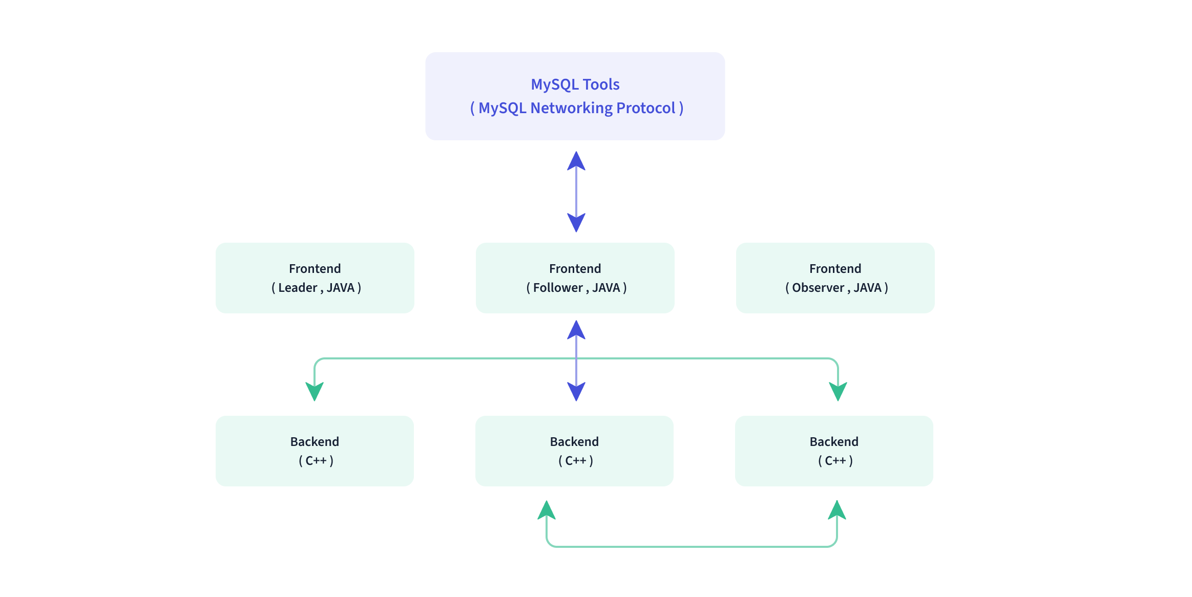
+
## Interface
@@ -82,11 +82,11 @@
Doris has an MPP-based query engine for parallel execution between and within nodes. It supports distributed shuffle join for large tables to better handle complicated queries.
-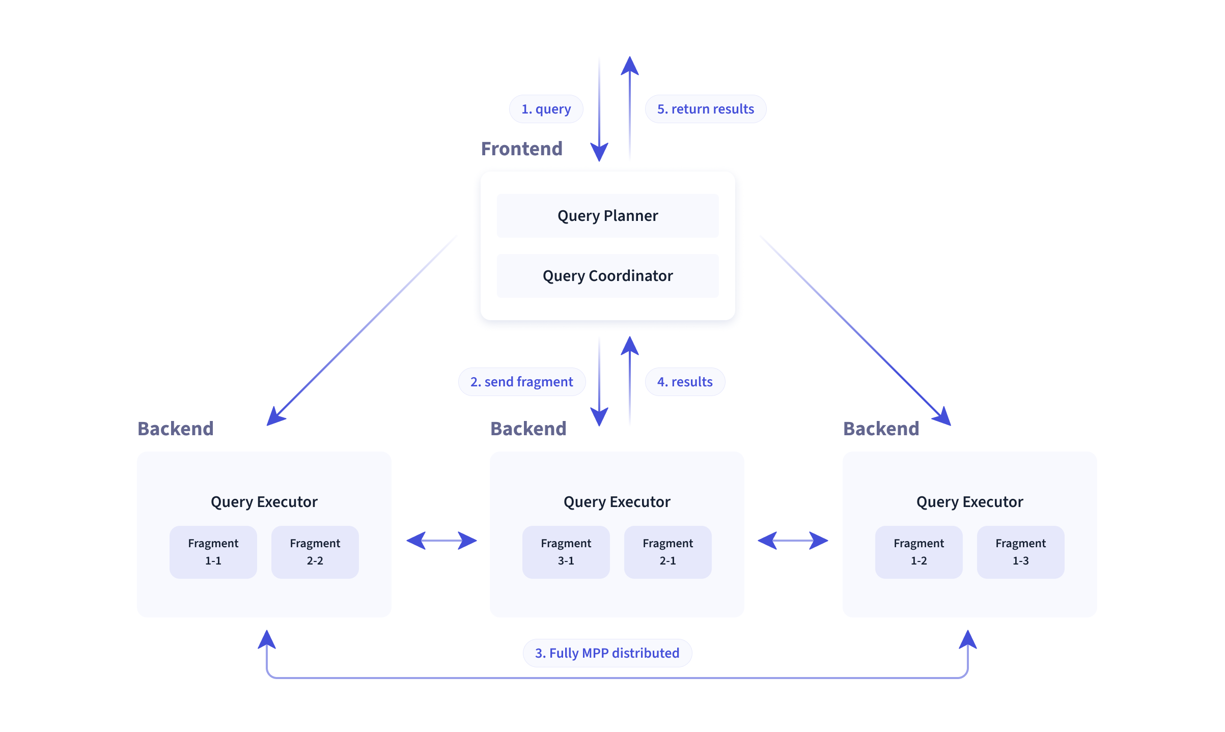
+
The Doris query engine is fully vectorized, with all memory structures laid out in a columnar format. This can largely reduce virtual function calls, increase cache hit rates, and make efficient use of SIMD instructions. Doris delivers a 5~10 times higher performance in wide table aggregation scenarios than non-vectorized engines.
-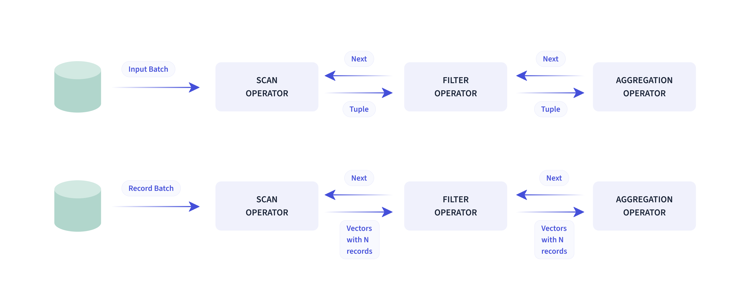
+
Doris uses **adaptive query execution** technology to dynamically adjust the execution plan based on runtime statistics. For example, it can generate a runtime filter and push it to the probe side. Specifically, it pushes the filters to the lowest-level scan node on the probe side, which largely reduces the data amount to be processed and increases join performance. The Doris runtime filter supports In/Min/Max/Bloom Filter.
diff --git a/docs/install/cluster-deployment/k8s-deploy/debug-crash.md b/docs/install/cluster-deployment/k8s-deploy/debug-crash.md
index 5e8de55..2c96041 100644
--- a/docs/install/cluster-deployment/k8s-deploy/debug-crash.md
+++ b/docs/install/cluster-deployment/k8s-deploy/debug-crash.md
@@ -64,7 +64,7 @@


-## 注意事项
+## Notes

 **After entering the pod, you need to modify the port information of the configuration file before you can manually start the corresponding Doris component.**
diff --git a/docs/lakehouse/lakehouse-overview.md b/docs/lakehouse/lakehouse-overview.md
index 0dfbec5..5644bd6 100644
--- a/docs/lakehouse/lakehouse-overview.md
+++ b/docs/lakehouse/lakehouse-overview.md
@@ -27,7 +27,9 @@
Before the integration of data lake and data warehouse, the history of data analysis went through three eras: database, data warehouse, and data lake analytics.
- Database, the fundamental concept, was primarily responsible for online transaction processing and providing basic data analysis capabilities.
+
- As data volumes grew, data warehouses emerged. They store valuable data that has been cleansed, processed, and modeled, providing analytics capabilities for business.
+
- The advent of data lakes was to serve the needs of enterprises for storing, managing, and reprocessing raw data. They required low-cost storage for structured, semi-structured, and even unstructured data, and they also needed an integrated solution encompassing data processing, data management, and data governance.
Data warehouses addresses the need for fast data analysis, while data lakes are good at data storage and management. The integration of them, known as "lakehouse", is to facilitate the seamless integration and free flow of data between the data lake and data warehouse. It enables users to leverage the analytic capabilities of the data warehouse while harnessing the data management power of the data lake.
@@ -37,8 +39,12 @@
We design the Doris lakehouse solution for the following four applicable scenarios:
- Lakehouse query acceleration: As a highly efficient OLAP query engine, Doris has excellent MPP-based vectorized distributed query capabilities. Data lake analysis with Doris will benefit from the efficient query engine.
+
- Unified data analysis gateway: Doris provides data query and writing capabilities for various and heterogeneous data sources. Users can unify these external data sources onto Doris' data mapping structure, allowing for a consistent query experience when accessing external data sources through Doris.
+
- Unified data integration: Doris, through its data lake integration capabilities, enables incremental or full data synchronization from multiple data sources to Doris. Doris processes the synchronized data and makes it available for querying. The processed data can also be exported to downstream systems as full or incremental data services. Using Doris, you can have less reliance on external tools and enable end-to-end connectivity from ata synchronization to data processing.
+
+
- More open data platform: Many data warehouses have their own storage formats. They require external data to be imported into themselve before the data queryable. This creates a closed ecosystem where data in the data warehouse can only be accessed by the data warehouse itself. In this case, users might concern if data will be locked into a specific data warehouse or wonder if there are any other easy way for data export. The Doris lakehouse solution provides open data formats, such as Parquet/ORC, to allow data access by various external systems. Additionally, just like Iceberg and Hudi providing open metadata management capabilities, metadata, whether stored in Doris, Hive Metastore, or other unified metadata centers, can be accessed through publicly available APIs. An open data ecosystem makes it easy for enterprises to migrate to new data management systems and reduces the costs and risks in this process.
## Doris-based data lakehouse architecture
@@ -50,8 +56,11 @@
**Data access steps:**
1. Create metadata mapping: Apache Doris fetches metadata via Catalog and caches it for metadata management. For metadata mapping, it supports JDBC username-password authentication, Kerberos/Ranger-based authentication, and KMS-based data encryption.
+
2. Launch query request: When the user launches a query request from the Doris frontend (FE), Doris generates a query plan based on its cached metadata. Then, it utilizes the Native Reader to fetch data from external storage (HDFS, S3) for data computation and analysis. During query execution, it caches the hot data to prepare for similar queries in the future.
+
3. Return result: When a query is finished, it returns the query result on the frontend.
+
4. Write result to data lake: For users who need to write the result back to the data lake instead of returning it on the frontend, Doris supports result writeback in CSV, Parquet, and ORC formats via the export method to the data lake.
## Core technologies
@@ -63,6 +72,7 @@
The data connection framework in Apache Doris includes metadata connection and data reading.
- Metadata connection: Metadata connection is conducted in the frontend of Doris. The MetaData Manager in the frontend can access and manage metadata from Hive Metastore, JDBC, and data files.
+
- Data reading: Apache Doris has a NativeReader for efficient data reading from HDFS and object storage. It supports Parquet, ORC, and text data. You can also connect Apache Doris to the Java big data ecosystem via its JNI Connector.

@@ -80,7 +90,9 @@
**Data caching**
- File caching: Apache Doris caches hot data from the data lake onto its local disks to reduce data transfer via the network and increase data access efficiency.
+
- Cache distribution: Apache Doris distributes the cached data across all backend nodes via consistent hashing to avoid cache expiration caused by cluster scaling.
+
- Cache eviction(update): When Apache Doris detects changes in the metadata of a data file, it promptly updates its cached data to ensure data consistency.

@@ -88,6 +100,7 @@
**Query result caching & partition caching**
- Query result caching: Apache Doris caches the results of previous SQL queries, so it can reuse them when similar queries are launched. It will read the corresponding result from the cache directly and return it to the client. This increases query efficiency and concurrency.
+
- Partition caching: Apache Doris allows you to cache part of your data partitions in the backend to increase query efficiency. For example, if you need the data from the past 7 days (counting today), you can cache the data from the previous 6 days and merge it with today's data. This can largely reduce real-time computation burden and increase speed.

@@ -95,6 +108,7 @@
### Native Reader
- Self-developed Native Reader to avoid data conversion: Apache Doris has its own columnar storage format, which is different from Parquet and ORC. To avoid overheads caused by data format conversion, we have built our own Native Reader for Parquet and ORC files.
+
- Lazy materialization: The Native Reader can utilize indexes and filters to improve data reading. For example, when the user needs to do filtering based on the ID column, what the Native Reader does is to read and filter the ID column, take note of the relevant row numbers, and then read the corresponding rows of the other columns based on the row numbers recorded. This reduces data scanning and speeds up data reading.

@@ -134,10 +148,15 @@
With Multi-Catalog, Doris now has a new three-tiered metadata hierarchy (catalog -> database -> table), which means users can connect to external data at the catalog level directly. Currently it supports external catalogs including:
- Apache Hive
+
- Apache Iceberg
+
- Apache Hudi
+
- Elasticsearch
+
- JDBC
+
- Apache Paimon(Incubating)
Multi-Catalog works as an additional and enhanced external table connection method. It helps users conduct multi-catalog federated queries quickly.
@@ -188,8 +207,9 @@
Syntax help: [CREATE CATALOG](../sql-manual/sql-statements/Data-Definition-Statements/Create/CREATE-CATALOG/)
-1. View Catalog
-2. View existing Catalogs via the `SHOW CATALOGS` command:
+2. View Catalog
+
+3. View existing Catalogs via the `SHOW CATALOGS` command:
```Plain
mysql> SHOW CATALOGS;
@@ -202,10 +222,12 @@
```
- [SHOW CATALOGS](../sql-manual/sql-statements/Show-Statements/SHOW-CATALOGS/)
+
- You can view the CREATE CATALOG statement via [SHOW CREATE CATALOG](../sql-manual/sql-statements/Show-Statements/SHOW-CREATE-CATALOG).
+
- You can modify the Catalog PROPERTIES via [ALTER CATALOG](../sql-manual/sql-statements/Data-Definition-Statements/Alter/ALTER-CATALOG).
-1. Switch Catalog
+4. Switch Catalog
Switch to the Hive Catalog using the `SWITCH` command, and view the databases in it:
@@ -228,7 +250,7 @@
Syntax help: [SWITCH](../sql-manual/sql-statements/Utility-Statements/SWITCH/)
-1. Use the Catalog
+5. Use the Catalog
After switching to the Hive Catalog, you can use the relevant features.
@@ -320,7 +342,9 @@
```
- The table is identified in the format of `catalog.database.table`. For example, `internal.db1.part` in the above snippet.
+
- If the target table is in the current Database of the current Catalog, `catalog` and `database` in the format can be omitted.
+
- You can use the `INSERT INTO` command to insert table data from the Hive Catalog into a table in the Internal Catalog. This is how you can import data from External Catalogs to the Internal Catalog:
```Plain
@@ -384,16 +408,18 @@
Users can refresh metadata in the following ways.
-#### Manual refresh
+**Manual refresh**
Users need to manually refresh the metadata through the [REFRESH](../sql-manual/sql-statements/Utility-Statements/REFRESH) command.
-#### Regular refresh
+**Regular refresh**
When creating the catalog, specify the refresh time parameter `metadata_refresh_interval_sec` in the properties. It is measured in seconds. If this is set when creating the catalog, the FE master node will refresh the catalog regularly accordingly. Currently, Doris supports regular refresh for three types of catalogs:
- hms: Hive MetaStore
+
- es: Elasticsearch
+
- Jdbc: standard interface for database access (JDBC)
```Plain
@@ -405,6 +431,6 @@
);
```
-#### Auto Refresh
+**Auto Refresh**
Currently Doris supports auto-refresh for [Hive](../lakehouse/datalake-analytics/hive) Catalog.
diff --git a/docs/query/duplicate/using-hll.md b/docs/query/duplicate/using-hll.md
index 2f98f52..2d91aa7 100644
--- a/docs/query/duplicate/using-hll.md
+++ b/docs/query/duplicate/using-hll.md
@@ -113,17 +113,17 @@
        -H "columns:dt,id,name,province,os, pv=hll_hash(id)" -T test_hll.csv http://fe_IP:8030/api/demo/test_hll/_stream_load
    ```

-   The sample data is as follows(test_hll.csv):
+   The sample data is as follows (test_hll.csv):

-   ```
-   2022-05-05,10001,测试01,北京,windows
-   2022-05-05,10002,测试01,北京,linux
-   2022-05-05,10003,测试01,北京,macos
-   2022-05-05,10004,测试01,河北,windows
-   2022-05-06,10001,测试01,上海,windows
-   2022-05-06,10002,测试01,上海,linux
-   2022-05-06,10003,测试01,江苏,macos
-   2022-05-06,10004,测试01,陕西,windows
+   ```text
+  2022-05-05,10001,Testing01,Beijing,Windows
+  2022-05-05,10002,Testing01,Beijing,Linux
+  2022-05-05,10003,Testing01,Beijing,MacOS
+  2022-05-05,10004,Testing01,Hebei,Windows
+  2022-05-06,10001,Testing01,Shanghai,Windows
+  2022-05-06,10002,Testing01,Shanghai,Linux
+  2022-05-06,10003,Testing01,Jiangsu,MacOS
+  2022-05-06,10004,Testing01,Shaanxi,Windows
    ```

    The import result is as follows:
diff --git a/docs/query/join-optimization/bucket-shuffle-join.md b/docs/query/join-optimization/bucket-shuffle-join.md
index 4a1775d..7f452b7 100644
--- a/docs/query/join-optimization/bucket-shuffle-join.md
+++ b/docs/query/join-optimization/bucket-shuffle-join.md
@@ -40,19 +40,19 @@
## Principle
The conventional distributed join methods supported by Doris is: `Shuffle Join, Broadcast Join`. Both of these join will lead to some network overhead.
-For example, there are join queries for table A and table B. the join method is hashjoin. The cost of different join types is as follows:
+For example, there are join queries for table A and table B. the join method is hashjoin. The cost of different join types is as follows:
* **Broadcast Join**: If table a has three executing hashjoinnodes according to the data distribution, table B needs to be sent to the three HashJoinNode. Its network overhead is `3B `, and its memory overhead is `3B`.
* **Shuffle Join**: Shuffle join will distribute the data of tables A and B to the nodes of the cluster according to hash calculation, so its network overhead is `A + B` and memory overhead is `B`.
The data distribution information of each Doris table is saved in FE. If the join statement hits the data distribution column of the left table, we should use the data distribution information to reduce the network and memory overhead of the join query. This is the source of the idea of bucket shuffle join.
-
+
The picture above shows how the Bucket Shuffle Join works. The SQL query is A table join B table. The equivalent expression of join hits the data distribution column of A. According to the data distribution information of table A. Bucket Shuffle Join sends the data of table B to the corresponding data storage and calculation node of table A. The cost of Bucket Shuffle Join is as follows:
-* network cost: ``` B < min(3B, A + B) ```
+* network cost: ``` B < min(3B, A + B) ```
-* memory cost: ``` B <= min(3B, B) ```
+* memory cost: ``` B <= min(3B, B) ```
Therefore, compared with Broadcast Join and Shuffle Join, Bucket shuffle join has obvious performance advantages. It reduces the time-consuming of data transmission between nodes and the memory cost of join. Compared with Doris's original join method, it has the following advantages
@@ -91,7 +91,7 @@
| | equal join conjunct: `test`.`k1` = `baseall`.`k1`
```
-The join type indicates that the join method to be used is:`BUCKET_SHUFFLE`。
+The join type indicates that the join method to be used is:`BUCKET_SHUFFLE`。
## Planning rules of Bucket Shuffle Join
diff --git a/docs/query/join-optimization/doris-join-optimization.md b/docs/query/join-optimization/doris-join-optimization.md
index 2b7d461..12e8def 100644
--- a/docs/query/join-optimization/doris-join-optimization.md
+++ b/docs/query/join-optimization/doris-join-optimization.md
@@ -32,15 +32,15 @@
## Doris Shuffle way
-1. Doris supports 4 Shuffle methods
+Doris supports 4 Shuffle methods
- 1. BroadCast Join
+1. BroadCast Join
- It requires the full data of the right table to be sent to the left table, that is, each node participating in Join has the full data of the right table, that is, T(R).
+ It requires the full data of the right table to be sent to the left table, that is, each node participating in Join has the full data of the right table, that is, T(R).
- Its applicable scenarios are more general, and it can support Hash Join and Nest loop Join at the same time, and its network overhead is N \* T(R).
+ Its applicable scenarios are more general, and it can support Hash Join and Nest loop Join at the same time, and its network overhead is N \* T(R).
- 
+ 
The data in the left table is not moved, and the data in the right table is sent to the scanning node of the data in the left table.
@@ -50,7 +50,7 @@
Its network overhead is: T(S) + T(R), but it can only support Hash Join, because it also calculates buckets according to the conditions of Join.
- 
+ 
The left and right table data are sent to different partition nodes according to the partition, and the calculated demerits are sent.
@@ -60,7 +60,7 @@
Its network overhead is: T(R) is equivalent to only Shuffle the data in the right table.
- 
+ 
The data in the left table does not move, and the data in the right table is sent to the node that scans the table in the left table according to the result of the partition calculation.
@@ -68,7 +68,7 @@
It is similar to Bucket Shuffle Join, which means that the data has been shuffled according to the preset Join column scenario when data is imported. Then the join calculation can be performed directly without considering the Shuffle problem of the data during the actual query.
- 
+ 
The data has been pre-partitioned, and the Join calculation is performed directly locally
@@ -96,12 +96,15 @@
Currently Doris supports three types of RuntimeFilter
- One is IN-IN, which is well understood, and pushes a hashset down to the data scanning node.
+
- The second is BloomFilter, which uses the data of the hash table to construct a BloomFilter, and then pushes the BloomFilter down to the scanning node that queries the data. .
+
- The last one is MinMax, which is a Range range. After the Range range is determined by the data in the right table, it is pushed down to the data scanning node.
There are two requirements for the applicable scenarios of Runtime Filter:
- The first requirement is that the right table is large and the left table is small, because building a Runtime Filter needs to bear the computational cost, including some memory overhead.
+
- The second requirement is that there are few results from the join of the left and right tables, indicating that this join can filter out most of the data in the left table.
When the above two conditions are met, turning on the Runtime Filter can achieve better results
@@ -112,31 +115,39 @@
### Runtime Filter Type
-- Doris provides three different Runtime Filter types:
- - The advantage of **IN** is that the effect filtering effect is obvious and fast. Its shortcomings are: First, it only applies to BroadCast. Second, when the right table exceeds a certain amount of data, it will fail. The current Doris configuration is 1024, that is, if the right table is larger than 1024, the Runtime Filter of IN will directly failed.
- - The advantage of **MinMax** is that the overhead is relatively small. Its disadvantage is that it has a relatively good effect on numeric columns, but basically no effect on non-numeric columns.
- - The feature of **Bloom Filter** is that it is universal, suitable for various types, and the effect is better. The disadvantage is that its configuration is more complicated and the calculation is high.
+Doris provides three different Runtime Filter types:
+- The advantage of **IN** is that the effect filtering effect is obvious and fast. Its shortcomings are: First, it only applies to BroadCast. Second, when the right table exceeds a certain amount of data, it will fail. The current Doris configuration is 1024, that is, if the right table is larger than 1024, the Runtime Filter of IN will directly failed.
-## Join Reader
+- The advantage of **MinMax** is that the overhead is relatively small. Its disadvantage is that it has a relatively good effect on numeric columns, but basically no effect on non-numeric columns.
+
+- The feature of **Bloom Filter** is that it is universal, suitable for various types, and the effect is better. The disadvantage is that its configuration is more complicated and the calculation is high.
+
+## Join Reorder
Once the database involves multi-table Join, the order of Join has a great impact on the performance of the entire Join query. Assuming that there are three tables to join, refer to the following picture, the left is the a table and the b table to do the join first, the intermediate result has 2000 rows, and then the c table is joined.
Next, look at the picture on the right and adjust the order of Join. Join the a table with the c table first, the intermediate result generated is only 100, and then finally join with the b table for calculation. The final join result is the same, but the intermediate result it generates has a 20x difference, which results in a big performance diff.
-
+
-- Doris currently supports the rule-based Join Reorder algorithm. Its logic is:
- - Make joins with large tables and small tables as much as possible, and the intermediate results it generates are as small as possible.
- - Put the conditional join table forward, that is to say, try to filter the conditional join table
- - Hash Join has higher priority than Nest Loop Join, because Hash Join itself is much faster than Nest Loop Join.
+Doris currently supports the rule-based Join Reorder algorithm. Its logic is:
+
+- Make joins with large tables and small tables as much as possible, and the intermediate results it generates are as small as possible.
+
+- Put the conditional join table forward, that is to say, try to filter the conditional join table
+
+- Hash Join has higher priority than Nest Loop Join, because Hash Join itself is much faster than Nest Loop Join.
## Doris Join optimization method
Doris Join tuning method:
- Use the Profile provided by Doris itself to locate the bottleneck of the query. Profile records various information in Doris' entire query, which is first-hand information for performance tuning. .
+
- Understand the Join mechanism of Doris, which is also the content shared with you in the second part. Only by knowing why and understanding its mechanism can we analyze why it is slow.
+
- Use Session variables to change some behaviors of Join, so as to realize the tuning of Join.
+
- Check the Query Plan to analyze whether this tuning is effective.
The above 4 steps basically complete a standard Join tuning process, and then it is to actually query and verify it to see what the effect is.
@@ -209,7 +220,11 @@
Finally, we summarize four suggestions for optimization and tuning of Doris Join:
- The first point: When doing Join, try to select columns of the same type or simple type. If the same type is used, reduce its data cast, and the simple type itself joins the calculation quickly.
+
- The second point: try to choose the Key column for Join. The reason is also introduced in the Runtime Filter. The Key column can play a better effect on delayed materialization.
+
- The third point: Join between large tables, try to make it Co-location, because the network overhead between large tables is very large, if you need to do Shuffle, the cost is very high.
+
- Fourth point: Use Runtime Filter reasonably, which is very effective in scenarios with high join filtering rate. But it is not a panacea, but has certain side effects, so it needs to be switched according to the granularity of specific SQL.
+
- Finally: When it comes to multi-table Join, it is necessary to judge the rationality of Join. Try to ensure that the left table is a large table and the right table is a small table, and then Hash Join will be better than Nest Loop Join. If necessary, you can use SQL Rewrite to adjust the order of Join using Hint.
diff --git a/docs/query/nereids/nereids.md b/docs/query/nereids/nereids.md
index 2e09e30..9895f1a 100644
--- a/docs/query/nereids/nereids.md
+++ b/docs/query/nereids/nereids.md
@@ -24,9 +24,7 @@
under the License.
-->
-# Nereids-the Brand New Planner
-<version since="dev"></version>
## R&D background
@@ -42,13 +40,13 @@
TPC-H SF100 query speed comparison. The environment is 3BE, the new optimizer uses the original SQL, and the statistical information is collected before executing the SQL. Old optimizers use hand-tuned SQL. It can be seen that the new optimizer does not need to manually optimize the query, and the overall query time is similar to that of the old optimizer after manual optimization.
-
+
-### more robust
+### More robust
All optimization rules of the new optimizer are completed on the logical execution plan tree. After the query syntax and semantic analysis is completed, it will be transformed into a tree structure. Compared with the internal data structure of the old optimizer, it is more reasonable and unified. Taking subquery processing as an example, the new optimizer is based on a new data structure, which avoids separate processing of subqueries by many rules in the old optimizer. In turn, the possibility of logic errors in optimization rules is reduced.
-### more flexible
+### More flexible
The architectural design of the new optimizer is more reasonable and modern. Optimization rules and processing stages can be easily extended. Can more quickly respond to user needs.
@@ -70,17 +68,24 @@
## Known issues and temporarily unsupported features
-### temporarily unsupported features
+### Temporarily unsupported features
-> If automatic fallback is enabled, it will automatically fall back to the old optimizer execution
+:::info Note
+If automatic fallback is enabled, it will automatically fall back to the old optimizer execution
+:::
-- Json、Array、Map and Struct types: The table in the query contains the above types, or the expressions in the query outputs the above types
+- Json, Array, Map and Struct types: The table in the query contains the above types, or the expressions in the query outputs the above types
+
- DML: Only support below DML statements: Insert Into Select, Update and Delete
+
- Matrialized view with predicates
+
- Function alias
+
- Java UDF and HDFS UDF
+
- High concurrent point query optimize
-### known issues
+### Known issues
- Cannot use partition cache to accelarate query
diff --git a/docs/query/udf/java-user-defined-function.md b/docs/query/udf/java-user-defined-function.md
index f1faffc..7108769 100644
--- a/docs/query/udf/java-user-defined-function.md
+++ b/docs/query/udf/java-user-defined-function.md
@@ -143,7 +143,7 @@

 When writing a UDAF using Java code, there are some required functions (marked as required) and an inner class State that must be implemented. Below is a specific example to illustrate.

-#### Example 1
+**Example 1**

 The following SimpleDemo will implement a simple function similar to sum, with the input parameter being INT and the output parameter being INT.

@@ -233,120 +233,121 @@

 ```

-#### Example 2
+**Example 2**

 ```java
-package org.apache.doris.udf.demo;
-
-
-import java.io.DataInputStream;
-import java.io.DataOutputStream;
-import java.math.BigDecimal;
-import java.util.Arrays;
-import java.util.logging.Logger;
-
-/*UDAF 计算中位数*/
-public class MedianUDAF {
-    Logger log = Logger.getLogger("MedianUDAF");
-
-    //状态存储
-    public static class State {
-        //返回结果的精度
-        int scale = 0;
-        //是否是某一个 tablet 下的某个聚合条件下的数据第一次执行 add 方法
-        boolean isFirst = true;
-        //数据存储
-        public StringBuilder stringBuilder;
-    }
-
-    //状态初始化
-    public State create() {
-        State state = new State();
-        //根据每个 tablet 下的聚合条件需要聚合的数据量大小,预先初始化,增加性能
-        state.stringBuilder = new StringBuilder(1000);
-        return state;
-    }
-
-
-    //处理执行单位处理各自 tablet 下的各自聚合条件下的每个数据
-    public void add(State state, Double val, int scale) {
-        try {
-            if (val != null && state.isFirst) {
-                state.stringBuilder.append(scale).append(",").append(val).append(",");
-                state.isFirst = false;
-            } else if (val != null) {
-                state.stringBuilder.append(val).append(",");
-            }
-        } catch (Exception e) {
-            //如果不能保证一定不会异常,建议每个方法都最大化捕获异常,因为目前不支持处理 java 抛出的异常
-            log.info("获取数据异常:" + e.getMessage());
-        }
-    }
-
-    //处理数据完需要输出等待聚合
-    public void serialize(State state, DataOutputStream out) {
-        try {
-            //目前暂时只提供 DataOutputStream,如果需要序列化对象可以考虑拼接字符串,转换 json,序列化成字节数组等方式
-            //如果要序列化 State 对象,可能需要自己将 State 内部类实现序列化接口
-            //最终都是要通过 DataOutputStream 传输
-            out.writeUTF(state.stringBuilder.toString());
-        } catch (Exception e) {
-            log.info("序列化异常:" + e.getMessage());
-        }
-    }
-
-    //获取处理数据执行单位输出的数据
-    public void deserialize(State state, DataInputStream in) {
-        try {
-            String string = in.readUTF();
-            state.scale = Integer.parseInt(String.valueOf(string.charAt(0)));
-            StringBuilder stringBuilder = new StringBuilder(string.substring(2));
-            state.stringBuilder = stringBuilder;
-        } catch (Exception e) {
-            log.info("反序列化异常:" + e.getMessage());
-        }
-    }
-
-    //聚合执行单位按照聚合条件合并某一个键下数据的处理结果 ,每个键第一次合并时,state1 参数是初始化的实例
-    public void merge(State state1, State state2) {
-        try {
-            state1.scale = state2.scale;
-            state1.stringBuilder.append(state2.stringBuilder.toString());
-        } catch (Exception e) {
-            log.info("合并结果异常:" + e.getMessage());
-        }
-    }
-
-    //对每个键合并后的数据进行并输出最终结果
-    public Double getValue(State state) {
-        try {
-            String[] strings = state.stringBuilder.toString().split(",");
-            double[] doubles = new double[strings.length + 1];
-            doubles = Arrays.stream(strings).mapToDouble(Double::parseDouble).toArray();
-
-            Arrays.sort(doubles);
-            double n = doubles.length - 1;
-            double index = n * 0.5;
-
-            int low = (int) Math.floor(index);
-            int high = (int) Math.ceil(index);
-
-            double value = low == high ? (doubles[low] + doubles[high]) * 0.5 : doubles[high];
-
-            BigDecimal decimal = new BigDecimal(value);
-            return decimal.setScale(state.scale, BigDecimal.ROUND_HALF_UP).doubleValue();
-        } catch (Exception e) {
-            log.info("计算异常:" + e.getMessage());
-        }
-        return 0.0;
-    }
-
-    //每个执行单位执行完都会执行
-    public void destroy(State state) {
-    }
-
+package org.apache.doris.udf.demo;
+
+import java.io.DataInputStream;
+import java.io.DataOutputStream;
+import java.math.BigDecimal;
+import java.util.Arrays;
+import java.util.logging.Logger;
+
+/* UDAF to calculate the median */
+public class MedianUDAF {
+    Logger log = Logger.getLogger("MedianUDAF");
+
+    // State storage
+    public static class State {
+        // Precision of the return result
+        int scale = 0;
+        // Whether it is the first time to execute the add method for a certain aggregation condition under a certain tablet
+        boolean isFirst = true;
+        // Data storage
+        public StringBuilder stringBuilder;
+    }
+
+    // Initialize the state
+    public State create() {
+        State state = new State();
+        // Pre-initialize based on the amount of data that needs to be aggregated under each aggregation condition of each tablet to increase performance
+        state.stringBuilder = new StringBuilder(1000);
+        return state;
+    }
+
+    // Process each data under respective aggregation conditions for each tablet
+    public void add(State state, Double val, int scale) {
+        try {
+            if (val != null && state.isFirst) {
+                state.stringBuilder.append(scale).append(",").append(val).append(",");
+                state.isFirst = false;
+            } else if (val != null) {
+                state.stringBuilder.append(val).append(",");
+            }
+        } catch (Exception e) {
+            // If it cannot be guaranteed that there will be no exceptions, it is recommended to maximize exception capture in each method, as handling of exceptions thrown by Java is currently not supported
+            log.info("Data acquisition exception: " + e.getMessage());
+        }
+    }
+
+    // Data needs to be output for aggregation after processing
+    public void serialize(State state, DataOutputStream out) {
+        try {
+            // Currently, only DataOutputStream is provided. If serialization of objects is required, methods such as concatenating strings, converting to JSON, or serializing into byte arrays can be considered
+            // If the State object needs to be serialized, it may be necessary to implement a serialization interface for the State inner class
+            // Ultimately, everything needs to be transmitted via DataOutputStream
+            out.writeUTF(state.stringBuilder.toString());
+        } catch (Exception e) {
+            log.info("Serialization exception: " + e.getMessage());
+        }
+    }
+
+    // Obtain the output data from the data processing execution unit
+    public void deserialize(State state, DataInputStream in) {
+        try {
+            String string = in.readUTF();
+            state.scale = Integer.parseInt(String.valueOf(string.charAt(0)));
+            StringBuilder stringBuilder = new StringBuilder(string.substring(2));
+            state.stringBuilder = stringBuilder;
+        } catch (Exception e) {
+            log.info("Deserialization exception: " + e.getMessage());
+        }
+    }
+
+    // The aggregation execution unit merges the processing results of data under certain aggregation conditions for a given key. The state1 parameter is the initialized instance during the first merge of each key
+    public void merge(State state1, State state2) {
+        try {
+            state1.scale = state2.scale;
+            state1.stringBuilder.append(state2.stringBuilder.toString());
+        } catch (Exception e) {
+            log.info("Merge result exception: " + e.getMessage());
+        }
+    }
+
+    // Output the final result after merging the data for each key
+    public Double getValue(State state) {
+        try {
+            String[] strings = state.stringBuilder.toString().split(",");
+            double[] doubles = new double[strings.length];
+            for (int i = 0; i < strings.length - 1; i++) {
+                doubles[i] = Double.parseDouble(strings[i + 1]);
+            }
+
+            Arrays.sort(doubles);
+            double n = doubles.length;
+            if (n == 0) {
+                return 0.0;
+            }
+            double index = (n - 1) / 2.0;
+
+            int low = (int) Math.floor(index);
+            int high = (int) Math.ceil(index);
+
+            double value = low == high ? (doubles[low] + doubles[high]) / 2 : doubles[high];
+
+            BigDecimal decimal = new BigDecimal(value);
+            return decimal.setScale(state.scale, BigDecimal.ROUND_HALF_UP).doubleValue();
+        } catch (Exception e) {
+            log.info("Calculation exception: " + e.getMessage());
+        }
+        return 0.0;
+    }
+
+    // Executed after each execution unit completes
+    public void destroy(State state) {
+    }
 }
-
 ```

 ### UDTF
diff --git a/docs/table-design/data-partition.md b/docs/table-design/data-partition.md
index 901b2da..5805199 100644
--- a/docs/table-design/data-partition.md
+++ b/docs/table-design/data-partition.md
@@ -24,44 +24,51 @@
 under the License.
 -->

-# Data Partition
+This document mainly introduces table creation and data partitioning in Doris, as well as potential problems and solutions encountered during table creation operations.

-This topic is about table creation and data partitioning in Doris, including the common problems in table creation and their solutions.
+## Basic concepts

-## Basic Concepts
-
-In Doris, data is logically described in the form of table.
+In Doris, data is logically described in the form of tables.

 ### Row & Column

-A table contains rows and columns.
+A table consists of rows and columns:

-Row refers to a row of user data. Column is used to describe different fields in a row of data.
+- Row: Represents a single line of user data;

-Columns can be divided into two categories: Key and Value. From a business perspective, Key and Value correspond to dimension columns and metric columns, respectively. The key column of Doris is the column specified in the table creation statement. The column after the keyword 'unique key' or 'aggregate key' or 'duplicate key' in the table creation statement is the key column, and the rest except the key column is the value column. In the Aggregate Model, rows with the same values in Key columns will be aggregated into one row. The way how Value columns are aggregated is specified by the user when the table is built. For more information about the Aggregate Model, please see the [Data Model](../table-design/data-model/overview.md).
+- Column: Used to describe different fields in a row of data;

-### Tablet & Partition
+- Columns can be divided into two types: Key and Value. From a business perspective, Key and Value can correspond to dimension columns and metric columns, respectively. The key columns in Doris are those specified in the table creation statement, which are the columns following the keywords `unique key`, `aggregate key`, or `duplicate key`. The remaining columns are value columns. From the perspective of the aggregation model, rows with the same Key columns will be aggregated into a single row. The aggregation method for value columns is specified by the user during table creation. For more information on aggregation models, refer to the Doris [Data Model](../table-design/data-model/overview).

-In the Doris storage engine, user data are horizontally divided into data tablets (also known as data buckets). Each tablet contains several rows of data. The data between the individual tablets do not intersect and is physically stored independently.
+### Partition & Tablet

-Tablets are logically attributed to different Partitions. One Tablet belongs to only one Partition, and one Partition contains several Tablets. Since the tablets are physically stored independently, the partitions can be seen as physically independent, too. Tablet is the smallest physical storage unit for data operations such as movement and replication.
+Doris supports two levels of data partitioning. The first level is Partitioning, which supports Range and List partition. The second level is Bucket (also known as Tablet), which supports Hash and Random . If no partitioning is established during table creation, Doris generates a default partition that is transparent to the user. When using the default partition, only Bucket is supported.

-A Table is formed of multiple Partitions. Partition can be thought of as the smallest logical unit of management. Data import and deletion can be performed on only one Partition.
+In the Doris storage engine, data is horizontally partitioned into several tablets. Each tablet contains several rows of data. There is no overlap between the data in different tablets, and they are stored physically independently.

-## Data Partitioning
+Multiple tablets logically belong to different partitions. A single tablet belongs to only one partition, while a partition contains several tablets. Because tablets are stored physically independently, partitions can also be considered physically independent. The tablet is the smallest physical storage unit for operations such as data movement and replication.

-The following illustrates on data partitioning in Doris using the example of a CREATE TABLE operation.
+Several partitions compose a table. The partition can be considered the smallest logical management unit.

-CREATE TABLE in Doris is a synchronous command. It returns results after the SQL execution is completed. Successful returns indicate successful table creation. For more information on the syntax, please refer to [CREATE TABLE](../sql-manual/sql-statements/Data-Definition-Statements/Create/CREATE-TABLE.md), or input  the `HELP CREATE TABLE;` command.
+Benefits of Two-Level data partitioning:

-This section introduces how to create tables in Doris.
+- For dimensions with time or similar ordered values, such dimension columns can be used as partitioning columns. The partition granularity can be evaluated based on import frequency and partition data volume.
+
+- Historical data deletion requirements: If there is a need to delete historical data (such as retaining only the data for the most recent several days), composite partition can be used to achieve this goal by deleting historical partitions. Alternatively, DELETE statements can be sent within specified partitions to delete data.
+
+- Solving data skew issues: Each partition can specify the number of buckets independently. For example, when partitioning by day and there are significant differences in data volume between days, the number of buckets for each partition can be specified to reasonably distribute data across different partitions. It is recommended to choose a column with high distinctiveness as the bucketing column.
+
+### Example of creating a table
+
+CREATE TABLE in Doris is a synchronous command. It returns results after the SQL execution is completed. Successful returns indicate successful table creation. For more information, please refer to [CREATE TABLE](../sql-manual/sql-statements/Data-Definition-Statements/Create/CREATE-TABLE), or input  the `HELP CREATE TABLE;` command.
+
+This section introduces how to create tables in Doris by range partiton and hash buckets.

 ```sql
 -- Range Partition
-
-CREATE TABLE IF NOT EXISTS example_db.example_range_tbl
+CREATE TABLE IF NOT EXISTS example_range_tbl
 (
-    `user_id` LARGEINT NOT NULL COMMENT "User ID",
+     `user_id` LARGEINT NOT NULL COMMENT "User ID",
     `date` DATE NOT NULL COMMENT "Date when the data are imported",
     `timestamp` DATETIME NOT NULL COMMENT "Timestamp when the data are imported",
     `city` VARCHAR(20) COMMENT "User location city",
@@ -70,436 +77,992 @@
     `last_visit_date` DATETIME REPLACE DEFAULT "1970-01-01 00:00:00" COMMENT "User last visit time",
     `cost` BIGINT SUM DEFAULT "0" COMMENT "Total user consumption",
     `max_dwell_time` INT MAX DEFAULT "0" COMMENT "Maximum user dwell time",
-    `min_dwell_time` INT MIN DEFAULT "99999" COMMENT "Minimum user dwell time"
+    `min_dwell_time` INT MIN DEFAULT "99999" COMMENT "Minimum user dwell time"
 )
-ENGINE=olap
+ENGINE=OLAP
 AGGREGATE KEY(`user_id`, `date`, `timestamp`, `city`, `age`, `sex`)
 PARTITION BY RANGE(`date`)
 (
-    PARTITION `p201701` VALUES LESS THAN ("2017-02-01"),
-    PARTITION `p201702` VALUES LESS THAN ("2017-03-01"),
-    PARTITION `p201703` VALUES LESS THAN ("2017-04-01"),
-    PARTITION `p2018` VALUES [("2018-01-01"), ("2019-01-01"))
+    PARTITION `p201701` VALUES [("2017-01-01"),  ("2017-02-01")),
+    PARTITION `p201702` VALUES [("2017-02-01"), ("2017-03-01")),
+    PARTITION `p201703` VALUES [("2017-03-01"), ("2017-04-01"))
 )
 DISTRIBUTED BY HASH(`user_id`) BUCKETS 16
 PROPERTIES
 (
-    "replication_num" = "3",
-    "storage_medium" = "SSD",
-    "storage_cooldown_time" = "2018-01-01 12:00:00"
+    "replication_num" = "1"
 );
+```

+Here use the AGGREGATE KEY data model as an example. In the AGGREGATE KEY data model, all columns that are specified with an aggregation type (SUM, REPLACE, MAX, or MIN) are Value columns. The rest are the Key columns.

--- List Partition
+In the PROPERTIES at the end of the CREATE TABLE statement, you can find detailed information about the relevant parameters that can be set in PROPERTIES by referring to the documentation on [CREATE TABLE](../sql-manual/sql-statements/Data-Definition-Statements/Create/CREATE-TABLE).

-CREATE TABLE IF NOT EXISTS example_db.example_list_tbl
+The default type of ENGINE is OLAP. In Doris, only this OLAP ENGINE type is responsible for data management and storage by Doris itself. Other ENGINE types, such as mysql, broker, es, etc., are essentially just mappings to tables in other external databases or systems, allowing Doris to read this data. However, Doris itself does not create, manage, or store any tables or data for non-OLAP ENGINE types.
+
+`IF NOT EXISTS` indicates that if the table has not been created before, it will be created. Note that this only checks if the table name exists and does not check if the schema of the new table is the same as the schema of an existing table. Therefore, if there is a table with the same name but a different schema, this command will also return successfully, but it does not mean that a new table and a new schema have been created.
+
+### View partition
+
+You can use the `show create table` command to view the partition information of a table.
+
+```sql
+> show create table  example_range_tbl
++-------------------+---------------------------------------------------------------------------------------------------------+
+| Table             | Create Table                                                                                            |
++-------------------+---------------------------------------------------------------------------------------------------------+
+| example_range_tbl | CREATE TABLE `example_range_tbl` (                                                                      |
+|                   |   `user_id` largeint(40) NOT NULL COMMENT 'User ID',                                                     |
+|                   |   `date` date NOT NULL COMMENT 'Date when the data are imported',                                                      |
+|                   |   `timestamp` datetime NOT NULL COMMENT 'Timestamp when the data are imported',                                             |
+|                   |   `city` varchar(20) NULL COMMENT 'User location city',                                                       |
+|                   |   `age` smallint(6) NULL COMMENT 'User age',                                                            |
+|                   |   `sex` tinyint(4) NULL COMMENT 'User gender',                                                             |
+|                   |   `last_visit_date` datetime REPLACE NULL DEFAULT "1970-01-01 00:00:00" COMMENT 'User last visit time', |
+|                   |   `cost` bigint(20) SUM NULL DEFAULT "0" COMMENT 'Total user consumption',                                          |
+|                   |   `max_dwell_time` int(11) MAX NULL DEFAULT "0" COMMENT 'Maximum user dwell time',                             |
+|                   |   `min_dwell_time` int(11) MIN NULL DEFAULT "99999" COMMENT 'Minimum user dwell time'                          |
+|                   | ) ENGINE=OLAP                                                                                           |
+|                   | AGGREGATE KEY(`user_id`, `date`, `timestamp`, `city`, `age`, `sex`)                                     |
+|                   | COMMENT 'OLAP'                                                                                          |
+|                   | PARTITION BY RANGE(`date`)                                                                              |
+|                   | (PARTITION p201701 VALUES [('0000-01-01'), ('2017-02-01')),                                             |
+|                   | PARTITION p201702 VALUES [('2017-02-01'), ('2017-03-01')),                                              |
+|                   | PARTITION p201703 VALUES [('2017-03-01'), ('2017-04-01')))                                              |
+|                   | DISTRIBUTED BY HASH(`user_id`) BUCKETS 16                                                               |
+|                   | PROPERTIES (                                                                                            |
+|                   | "replication_allocation" = "tag.location.default: 1",                                                   |
+|                   | "is_being_synced" = "false",                                                                            |
+|                   | "storage_format" = "V2",                                                                                |
+|                   | "light_schema_change" = "true",                                                                         |
+|                   | "disable_auto_compaction" = "false",                                                                    |
+|                   | "enable_single_replica_compaction" = "false"                                                            |
+|                   | );                                                                                                      |
++-------------------+---------------------------------------------------------------------------------------------------------+
+```
+
+You can use `show partitions from your_table` command to view the partition information of a table.
+
+```
+> show partitions from example_range_tbl
++-------------+---------------+----------------+---------------------+--------+--------------+--------------------------------------------------------------------------------+-----------------+---------+----------------+---------------
++---------------------+---------------------+--------------------------+----------+------------+-------------------------+-----------+
+| PartitionId | PartitionName | VisibleVersion | VisibleVersionTime  | State  | PartitionKey | Range                                                                          | DistributionKey | Buckets | ReplicationNum | StorageMedium
+| CooldownTime        | RemoteStoragePolicy | LastConsistencyCheckTime | DataSize | IsInMemory | ReplicaAllocation       | IsMutable |
++-------------+---------------+----------------+---------------------+--------+--------------+--------------------------------------------------------------------------------+-----------------+---------+----------------+---------------
++---------------------+---------------------+--------------------------+----------+------------+-------------------------+-----------+
+| 28731       | p201701       | 1              | 2024-01-25 10:50:51 | NORMAL | date         | [types: [DATEV2]; keys: [0000-01-01]; ..types: [DATEV2]; keys: [2017-02-01]; ) | user_id         | 16      | 1              | HDD
+| 9999-12-31 23:59:59 |                     |                    | 0.000    | false      | tag.location.default: 1 | true      |
+| 28732       | p201702       | 1              | 2024-01-25 10:50:51 | NORMAL | date         | [types: [DATEV2]; keys: [2017-02-01]; ..types: [DATEV2]; keys: [2017-03-01]; ) | user_id         | 16      | 1              | HDD
+| 9999-12-31 23:59:59 |                     |                    | 0.000    | false      | tag.location.default: 1 | true      |
+| 28733       | p201703       | 1              | 2024-01-25 10:50:51 | NORMAL | date         | [types: [DATEV2]; keys: [2017-03-01]; ..types: [DATEV2]; keys: [2017-04-01]; ) | user_id         | 16      | 1              | HDD
+| 9999-12-31 23:59:59 |                     |                    | 0.000    | false      | tag.location.default: 1 | true      |
++-------------+---------------+----------------+---------------------+--------+--------------+--------------------------------------------------------------------------------+-----------------+---------+----------------+---------------
++---------------------+---------------------+--------------------------+----------+------------+-------------------------+-----------+
+```
+
+### Alter partition
+
+You can add a new partition by using the `alter table add partition` command.
+
+```sql
+ALTER TABLE example_range_tbl ADD  PARTITION p201704 VALUES LESS THAN("2020-05-01") DISTRIBUTED BY HASH(`user_id`) BUCKETS 5;
+```
+
+For more partition modification operations, please refer to the SQL manual on [ALTER-TABLE-PARTITION](../sql-manual/sql-statements/Data-Definition-Statements/Alter/ALTER-TABLE-PARTITION).
+
+## Manual partitioning
+
+### Partition columns
+
+- Partition columns can be specified as one or multiple columns, and the partition columns must be KEY columns. The usage of multi-column partitioning will be introduced later in the summary section of multi-column partitioning.
+
+- When `allowPartitionColumnNullable` is set to true, Range partition supports the use of NULL partition columns. List Partition does not support NULL partition columns at all times.
+
+- Regardless of the type of partition column, double quotes are required when writing partition values.
+
+- There is theoretically no upper limit on the number of partitions.
+
+- When creating a table without partitioning, the system will automatically generate a full-range partition with the same name as the table name. This partition is not visible to users and cannot be deleted or modified.
+
+- Overlapping ranges are not allowed when creating partitions.
+
+### Range partition
+
+Partition columns are usually time columns for convenient management of old and new data. Range partition supports column types such as DATE, DATETIME, TINYINT, SMALLINT, INT, BIGINT, and LARGEINT.
+
+Partition information supports four writing methods:
+
+- FIXED RANGE: the partition as a left-closed, right-open interval.
+
+```sql
+PARTITION BY RANGE(col1[, col2, ...])
+(
+    PARTITION partition_name1 VALUES [("k1-lower1", "k2-lower1", "k3-lower1",...), ("k1-upper1", "k2-upper1", "k3-upper1", ...)),
+    PARTITION partition_name2 VALUES [("k1-lower1-2", "k2-lower1-2", ...), ("k1-upper1-2", MAXVALUE, ))
+)
+```
+
+For example:
+
+```
+PARTITION BY RANGE(`date`)
 (
-    `user_id` LARGEINT NOT NULL COMMENT "User ID",
-    `date` DATE NOT NULL COMMENT "Date when the data are imported",
-    `timestamp` DATETIME NOT NULL COMMENT "Timestamp when the data are imported",
-    `city` VARCHAR(20) NOT NULL COMMENT "User location city",
-    `age` SMALLINT COMMENT "User Age",
-    `sex` TINYINT COMMENT "User gender",
-    `last_visit_date` DATETIME REPLACE DEFAULT "1970-01-01 00:00:00" COMMENT "User last visit time",
-    `cost` BIGINT SUM DEFAULT "0" COMMENT "Total user consumption",
-    `max_dwell_time` INT MAX DEFAULT "0" COMMENT "Maximum user dwell time",
-    `min_dwell_time` INT MIN DEFAULT "99999" COMMENT "Minimum user dwell time"
+    PARTITION `p201701` VALUES [("2017-01-01"),  ("2017-02-01")),
+    PARTITION `p201702` VALUES [("2017-02-01"), ("2017-03-01")),
+    PARTITION `p201703` VALUES [("2017-03-01"), ("2017-04-01"))
 )
-ENGINE=olap
-AGGREGATE KEY(`user_id`, `date`, `timestamp`, `city`, `age`, `sex`)
-PARTITION BY LIST(`city`)
+```
+
+- LESS THAN: Only define the upper bound of the partition. The lower bound is determined by the upper bound of the previous partition.
+
+```sql
+PARTITION BY RANGE(col1[, col2, ...])
+(
+    PARTITION partition_name1 VALUES LESS THAN MAXVALUE | ("value1", "value2", ...),
+    PARTITION partition_name2 VALUES LESS THAN MAXVALUE | ("value1", "value2", ...)
+)
+```
+
+For example:
+
+```sql
+PARTITION BY RANGE(`date`)
+(
+    PARTITION `p201701` VALUES LESS THAN ("2017-02-01"),
+    PARTITION `p201702` VALUES LESS THAN ("2017-03-01"),
+    PARTITION `p201703` VALUES LESS THAN ("2017-04-01")
+)
+
+PARTITION BY RANGE(`date`)
+(
+    PARTITION `p201701` VALUES LESS THAN ("2017-02-01"),
+    PARTITION `p201702` VALUES LESS THAN ("2017-03-01"),
+    PARTITION `p201703` VALUES LESS THAN ("2017-04-01")
+    PARTITION `other` VALUES LESS THAN (MAXVALUE)
+)
+```
+
+- BATCH RANGE: Batch create RANGE partitions of numeric and time types, defining the partitions as left-closed, right-open intervals, and setting the step size.
+
+```sql
+PARTITION BY RANGE(int_col)
+(
+    FROM (start_num) TO (end_num) INTERVAL interval_value
+)
+
+PARTITION BY RANGE(date_col)
+(
+    FROM ("start_date") TO ("end_date") INTERVAL num YEAR | num MONTH | num WEEK | num DAY | 1 HOUR
+)
+```
+
+For example:
+
+```sql
+PARTITION BY RANGE(age)
+(
+    FROM (1) TO (100) INTERVAL 10
+)
+
+PARTITION BY RANGE(`date`)
+(
+    FROM ("2000-11-14") TO ("2021-11-14") INTERVAL 2 YEAR
+)
+```
+
+- MULTI RANGE: Batch create RANGE partitions, defining the partitions as left-closed, right-open intervals. For example:
+
+```sql
+PARTITION BY RANGE(col)
+(
+   FROM ("2000-11-14") TO ("2021-11-14") INTERVAL 1 YEAR,
+   FROM ("2021-11-14") TO ("2022-11-14") INTERVAL 1 MONTH,
+   FROM ("2022-11-14") TO ("2023-01-03") INTERVAL 1 WEEK,
+   FROM ("2023-01-03") TO ("2023-01-14") INTERVAL 1 DAY,
+   PARTITION p_20230114 VALUES [('2023-01-14'), ('2023-01-15'))
+)
+```
+
+### List partition
+
+Partition columns support data types such as BOOLEAN, TINYINT, SMALLINT, INT, BIGINT, LARGEINT, DATE, DATETIME, CHAR, and VARCHAR. Partition values are enumerated values. Only when the data is one of the enumerated values of the target partition, the partition can be hit .
+
+Partitions support specifying the enumerated values contained in each partition through VALUES IN (...).
+
+For example:
+
+```sql
+PARTITION BY LIST(city)
 (
     PARTITION `p_cn` VALUES IN ("Beijing", "Shanghai", "Hong Kong"),
     PARTITION `p_usa` VALUES IN ("New York", "San Francisco"),
     PARTITION `p_jp` VALUES IN ("Tokyo")
 )
-DISTRIBUTED BY HASH(`user_id`) BUCKETS 16
+```
+
+List partition also supports multi-column partitioning, for example:
+
+```sql
+PARTITION BY LIST(id, city)
+(
+    PARTITION p1_city VALUES IN (("1", "Beijing"), ("1", "Shanghai")),
+    PARTITION p2_city VALUES IN (("2", "Beijing"), ("2", "Shanghai")),
+    PARTITION p3_city VALUES IN (("3", "Beijing"), ("3", "Shanghai"))
+)
+```
+
+## Dynamic partition
+
+Dynamic partition is designed to manage partition's Time-to-Life (TTL), reducing the burden on users.
+
+In some usage scenarios, the user will partition the table according to the day and perform routine tasks regularly every day. At this time, the user needs to manually manage the partition. Otherwise, the data load may fail because the user does not create a partition. This brings additional maintenance costs to the user.
+
+With dynamic partitioning, users can define rules for partition creation and deletion when establishing tables. The FE initiates a background thread to handle partition creation or deletion based on these user-defined rules. Users also have the flexibility to modify these rules during runtime.
+
+It's important to note that dynamic partitioning is exclusively supported by range partitions. Currently, the functionality enables dynamic addition and deletion of partitions.
+
+:::tip
+
+This feature will be disabled when synchronized by CCR. If this table is copied by CCR, that is, PROPERTIES contains `is_being_synced = true`, it will be displayed as enabled in show create table, but will not actually take effect. When `is_being_synced` is set to `false`, these features will resume working, but the `is_being_synced` property is for CCR peripheral modules only and should not be manually set during CCR synchronization.
+
+:::
+
+### How to use
+
+The rules for dynamic partitioning can be specified when the table is created or modified at runtime.
+
+Currently, dynamic partition rules can only be set for partition tables with single partition columns.
+
+- Specified when creating table
+
+```sql
+CREATE TABLE tbl1
+(...)
 PROPERTIES
 (
-    "replication_num" = "3",
-    "storage_medium" = "SSD",
-    "storage_cooldown_time" = "2018-01-01 12:00:00"
-);
-
+    "dynamic_partition.prop1" = "value1",
+    "dynamic_partition.prop2" = "value2",
+    ...
+)
 ```

-### Definition of Column
+- Modify at runtime

-Here we only use the AGGREGATE KEY data model as an example. See [Doris Data Model](../table-design/data-model/overview) for more information.
+```sql
+ALTER TABLE tbl1 SET
+(
+    "dynamic_partition.prop1" = "value1",
+    "dynamic_partition.prop2" = "value2",
+    ...
+)
+```

-You can view the basic types of columns by executing `HELP CREATE TABLE;` in MySQL Client.
+### Rule parameters

-In the AGGREGATE KEY data model, all columns that are specified with an aggregation type (SUM, REPLACE, MAX, or MIN) are Value columns. The rest are the Key columns.
+The rules of dynamic partition are prefixed with `dynamic_partition.`:

-A few suggested rules for defining columns include:
+- `dynamic_partition.enable`

-1. The Key columns must precede all Value columns.
-2. Try to choose the INT type as much as possible. Because calculations and lookups on INT types are much more efficient than those on strings.
-3. For the lengths of the INT types, follow the **good enough** principle.
-4. For the lengths of the VARCHAR and STRING types, also follow the **good enough** principle.
+  Whether to enable the dynamic partition feature. Can be specified as `TRUE` or` FALSE`. If not filled, the default is `TRUE`. If it is `FALSE`, Doris will ignore the dynamic partitioning rules of the table.

-### Partitioning and Bucketing
+- `dynamic_partition.time_unit`(required parameters)

-Doris supports two layers of data partitioning. The first level is Partition, including range partitioning and list partitioning. The second is Bucket (Tablet), including hash and random partitioning.
+  The unit for dynamic partition scheduling. Can be specified as `HOUR`,`DAY`,` WEEK`, `MONTH` and `YEAR`, means to create or delete partitions by hour, day, week, month and year, respectively.

-It is also possible to use one layer of data partitioning, If you do not write the partition statement when creating the table, Doris will generate a default partition at this time, which is transparent to the user. In this case, it only supports data bucketing.
+  When specified as `HOUR`, the suffix format of the dynamically created partition name is `yyyyMMddHH`, for example, `2020032501`. *When the time unit is HOUR, the data type of partition column cannot be DATE.*

-1. Partition
+  When specified as `DAY`, the suffix format of the dynamically created partition name is `yyyyMMdd`, for example, `20200325`.

-   * You can specify one or more columns as the partitioning columns, but they have to be KEY columns. The usage of multi-column partitions is described further below.
-   * Range Partition supports the use of NULL partition columns when `allowPartitionColumnNullable` is `true`. List Partition never supports NULL partition columns.
-   * Regardless of the type of the partitioning columns, double quotes are required for partition values.
-   * There is no theoretical limit on the number of partitions.
-   * If users create a table without specifying the partitions, the system will automatically generate a Partition with the same name as the table. This Partition contains all data in the table and is neither visible to users nor modifiable.
-   * **Partitions should not have overlapping ranges**.
+  When specified as `WEEK`, the suffix format of the dynamically created partition name is `yyyy_ww`. That is, the week of the year of current date. For example, the suffix of the partition created for `2020-03-25` is `2020_13`, indicating that it is currently the 13th week of 2020.

-   #### Range Partitioning
+  When specified as `MONTH`, the suffix format of the dynamically created partition name is `yyyyMM`, for example, `202003`.

-   * Partitioning columns are usually time columns for easy management of old and new data.
+  When specified as `YEAR`, the suffix format of the dynamically created partition name is `yyyy`, for example, `2020`.

-   * Range partitioning support column type: [DATE,DATETIME,TINYINT,SMALLINT,INT,BIGINT,LARGEINT]
+- `dynamic_partition.time_zone`

-   * Range partitioning supports specifying only the upper bound by `VALUES LESS THAN (...)`. The system will use the upper bound of the previous partition as the lower bound of the next partition, and generate a left-closed right-open interval. It also supports specifying both the upper and lower bounds by `VALUES [...)`, and generate a left-closed right-open interval.
+  The time zone of the dynamic partition, if not filled in, defaults to the time zone of the current machine's system, such as `Asia/Shanghai`, if you want to know the supported TimeZone, you can found in [Timezone](https://en.wikipedia.org/wiki/List_of_tz_database_time_zones).

-   * The following takes the `VALUES [...)` method as an example since it is more comprehensible. It shows how the partition ranges change as we use the  `VALUES LESS THAN (...)` statement to add or delete partitions:
+- `dynamic_partition.start`

-     * As in the `example_range_tbl` example above, when the table is created, the following 3 partitions are automatically generated:
+  The starting offset of the dynamic partition, usually a negative number. Depending on the `time_unit` attribute, based on the current day (week / month), the partitions with a partition range before this offset will be deleted. If not filled, the default is `-2147483648`, that is, the history partition will not be  deleted.

-       ```
-       P201701: [MIN_VALUE, 2017-02-01)
-       P201702: [2017-02-01, 2017-03-01)
-       P201703: [2017-03-01, 2017-04-01)
-       ```
+- `dynamic_partition.end`(required parameters)

-     * If we add Partition p201705 VALUES LESS THAN ("2017-06-01"), the results will be as follows:
+  The end offset of the dynamic partition, usually a positive number. According to the difference of the `time_unit` attribute, the partition of the corresponding range is created in advance based on the current day (week / month).

-       ```
-       P201701: [MIN_VALUE, 2017-02-01)
-       P201702: [2017-02-01, 2017-03-01)
-       P201703: [2017-03-01, 2017-04-01)
-       P201705: [2017-04-01, 2017-06-01)
-       ```

-     * Then we delete Partition p201703, the results will be as follows:
+- `dynamic_partition.prefix`(required parameters)

-       ```
-       p201701: [MIN_VALUE, 2017-02-01)
-       p201702: [2017-02-01, 2017-03-01)
-       p201705: [2017-04-01, 2017-06-01)
-       ```
+  The dynamically created partition name prefix.

-       > Note that the partition range of p201702 and p201705 has not changed, and there is a gap between the two partitions: [2017-03-01, 2017-04-01). That means, if the imported data is within this gap range, the import would fail.

-     * Now we go on and delete Partition p201702, the results will be as follows:
+- `dynamic_partition.buckets`

-       ```
-       p201701: [MIN_VALUE, 2017-02-01)
-       p201705: [2017-04-01, 2017-06-01)
-       ```
+    The number of buckets corresponding to the dynamically created partitions.

-       > The gap range expands to: [2017-02-01, 2017-04-01)
+- `dynamic_partition.replication_num`

-     * Then we add Partition p201702new VALUES LESS THAN ("2017-03-01"), the results will be as follows:
+  The replication number of dynamic partition.If not filled in, defaults to the number of table's replication number.

-       ```
-       p201701: [MIN_VALUE, 2017-02-01)
-       p201702new: [2017-02-01, 2017-03-01)
-       p201705: [2017-04-01, 2017-06-01)
-       ```
+- `dynamic_partition.start_day_of_week`

-       > The gap range shrinks to: [2017-03-01, 2017-04-01)
+  When `time_unit` is` WEEK`, this parameter is used to specify the starting point of the week. The value ranges from 1 to 7. Where 1 is Monday and 7 is Sunday. The default is 1, which means that every week starts on Monday.

-     * Now we delete Partition p201701 and add Partition p201612 VALUES LESS THAN ("2017-01-01"), the partition result is as follows:

-       ```
-       p201612: [MIN_VALUE, 2017-01-01)
-       p201702new: [2017-02-01, 2017-03-01)
-       p201705: [2017-04-01, 2017-06-01)
-       ```
+- `dynamic_partition.start_day_of_month`

-       > This results in a new gap range: [2017-01-01, 2017-02-01)
+  When `time_unit` is` MONTH`, this parameter is used to specify the start date of each month. The value ranges from 1 to 28. 1 means the 1st of every month, and 28 means the 28th of every month. The default is 1, which means that every month starts at 1st. The 29, 30 and 31 are not supported at the moment to avoid ambiguity caused by lunar years or months.

-   In summary, the deletion of a partition does not change the range of the existing partitions, but might result in gaps. When a partition is added via the `VALUES LESS THAN` statement, the lower bound of one partition is the upper bound of its previous partition.

-   In addition to the single-column partitioning mentioned above, Range Partitioning also supports **multi-column partitioning**. Examples are as follows:
+- `dynamic_partition.create_history_partition`

-   ```text
-    PARTITION BY RANGE(`date`, `id`)
-    (
-        PARTITION `p201701_1000` VALUES LESS THAN ("2017-02-01", "1000"),
-        PARTITION `p201702_2000` VALUES LESS THAN ("2017-03-01", "2000"),
-        PARTITION `p201703_all` VALUES LESS THAN ("2017-04-01")
-    )
+  The default is false. When set to true, Doris will automatically create all partitions, as described in the creation rules below. At the same time, the parameter `max_dynamic_partition_num` of FE will limit the total number of partitions to avoid creating too many partitions at once. When the number of partitions expected to be created is greater than `max_dynamic_partition_num`, the operation will fail.
+
+  When the `start` attribute is not specified, this parameter has no effect.
+
+- `dynamic_partition.history_partition_num`
+
+  When `create_history_partition` is `true`, this parameter is used to specify the number of history partitions. The default value is -1, which means it is not set.
+
+- `dynamic_partition.hot_partition_num`
+
+  Specify how many of the latest partitions are hot partitions. For hot partition, the system will automatically set its `storage_medium` parameter to SSD, and set `storage_cooldown_time`.
+
+  :::tip
+
+  If there is no SSD disk path under the storage path, configuring this parameter will cause dynamic partition creation to fail.
+
+  :::
+
+  `hot_partition_num` is all partitions in the previous n days and in the future.
+
+  Let us give an example. Suppose today is 2021-05-20, partition by day, and the properties of dynamic partition are set to: hot_partition_num=2, end=3, start=-3. Then the system will automatically create the following partitions, and set the `storage_medium` and `storage_cooldown_time` properties:
+
+  ```sql
+  p20210517: ["2021-05-17", "2021-05-18") storage_medium=HDD storage_cooldown_time=9999-12-31 23:59:59
+  p20210518: ["2021-05-18", "2021-05-19") storage_medium=HDD storage_cooldown_time=9999-12-31 23:59:59
+  p20210519: ["2021-05-19", "2021-05-20") storage_medium=SSD storage_cooldown_time=2021-05-21 00:00:00
+  p20210520: ["2021-05-20", "2021-05-21") storage_medium=SSD storage_cooldown_time=2021-05-22 00:00:00
+  p20210521: ["2021-05-21", "2021-05-22") storage_medium=SSD storage_cooldown_time=2021-05-23 00:00:00
+  p20210522: ["2021-05-22", "2021-05-23") storage_medium=SSD storage_cooldown_time=2021-05-24 00:00:00
+  p20210523: ["2021-05-23", "2021-05-24") storage_medium=SSD storage_cooldown_time=2021-05-25 00:00:00
+  ```
+
+
+- `dynamic_partition.reserved_history_periods`
+
+  The range of reserved history periods. It should be in the form of `[yyyy-MM-dd,yyyy-MM-dd],[...,...]` while the `dynamic_partition.time_unit` is "DAY, WEEK, MONTH and YEAR". And it should be in the form of `[yyyy-MM-dd HH:mm:ss,yyyy-MM-dd HH:mm:ss],[...,...]` while the dynamic_partition.time_unit` is "HOUR". And no more spaces expected. The default value is `"NULL"`, which means it is not set.
+
+  Let us give an example. Suppose today is 2021-09-06, partitioned by day, and the properties of dynamic partition are set to:
+
+  ```time_unit="DAY/WEEK/MONTH/YEAR", end=3, start=-3, reserved_history_periods="[2020-06-01,2020-06-20],[2020-10-31,2020-11-15]"```.
+
+  The system will automatically reserve following partitions in following period :
+
+  ```sql
+  ["2020-06-01","2020-06-20"],
+  ["2020-10-31","2020-11-15"]
+  ```
+
+  or
+
+  ```time_unit="HOUR", end=3, start=-3, reserved_history_periods="[2020-06-01 00:00:00,2020-06-01 03:00:00]"```.
+
+  The system will automatically reserve following partitions in following period :
+
+  ```
+  ["2020-06-01 00:00:00","2020-06-01 03:00:00"]
+  ```
+
+  Otherwise, every `[...,...]` in `reserved_history_periods` is a couple of properties, and they should be set at the same time. And the first date can't be larger than the second one.
+
+
+- `dynamic_partition.storage_medium`
+
+
+  :::info Note
+  This parameteres is supported since Doris version 1.2.3
+  :::
+
+  Specifies the default storage medium for the created dynamic partition. HDD is the default, SSD can be selected.
+
+  Note that when set to SSD, the `hot_partition_num` property will no longer take effect, all partitions will default to SSD storage media and the cooldown time will be 9999-12-31 23:59:59.
+
+#### Create history partition rules
+
+When `create_history_partition` is `true`, i.e. history partition creation is enabled, Doris determines the number of history partitions to be created based on `dynamic_partition.start` and `dynamic_partition.history_partition_num`.
+
+Assuming the number of history partitions to be created is `expect_create_partition_num`, the number is as follows according to different settings.
+
+- `create_history_partition` = `true`
+
+  - `dynamic_partition.history_partition_num` is not set, i.e. -1.
+    `expect_create_partition_num` = `end` - `start`;
+
+  - `dynamic_partition.history_partition_num` is set
+    `expect_create_partition_num` = `end` - max(`start`, `-history_partition_num`);
+
+- `create_history_partition` = `false`
+
+No history partition will be created, `expect_create_partition_num` = `end` - 0;
+
+When `expect_create_partition_num` is greater than `max_dynamic_partition_num` (default 500), creating too many partitions is prohibited.
+
+**Examples:**
+
+Suppose today is 2021-05-20, partition by day, and the attributes of dynamic partition are set to `create_history_partition=true, end=3, start=-3, history_partition_num=1`, then the system will automatically create the following partitions.
+
+```
+p20210519
+p20210520
+p20210521
+p20210522
+p20210523
+```
+
+`history_partition_num=5` and keep the rest attributes as in 1, then the system will automatically create the following partitions.
+
+```
+p20210517
+p20210518
+p20210519
+p20210520
+p20210521
+p20210522
+p20210523
+```
+
+`history_partition_num=-1` i.e., if you do not set the number of history partitions and keep the rest of the attributes as in 1, the system will automatically create the following partitions.
+
+```
+p20210517
+p20210518
+p20210519
+p20210520
+p20210521
+p20210522
+p20210523
+```
+
+### Example
+
+1. Table `tbl1` partition column k1, type is DATE, create a dynamic partition rule. By day partition, only the partitions of the last 7 days are kept, and the partitions of the next 3 days are created in advance.
+
+   ```
+   CREATE TABLE tbl1
+   (
+       k1 DATE,
+       ...
+   )
+   PARTITION BY RANGE(k1) ()
+   DISTRIBUTED BY HASH(k1)
+   PROPERTIES
+   (
+       "dynamic_partition.enable" = "true",
+       "dynamic_partition.time_unit" = "DAY",
+       "dynamic_partition.start" = "-7",
+       "dynamic_partition.end" = "3",
+       "dynamic_partition.prefix" = "p",
+       "dynamic_partition.buckets" = "32"
+   );
    ```

-    In the above example, we specify `date` (DATE type) and `id` (INT type) as the partitioning columns, so the resulting partitions will be as follows:
+   Suppose the current date is 2020-05-29. According to the above rules, tbl1 will produce the following partitions:

-    ``` text
-        *p201701_1000: [(MIN_VALUE, MIN_VALUE), ("2017-02-01", "1000") )
-        *p201702_2000: [("2017-02-01", "1000"), ("2017-03-01", "2000") )
-        *p201703_all: [("2017-03-01", "2000"), ("2017-04-01", MIN_VALUE))
-    ```
+   ```
+   p20200529: ["2020-05-29", "2020-05-30")
+   p20200530: ["2020-05-30", "2020-05-31")
+   p20200531: ["2020-05-31", "2020-06-01")
+   p20200601: ["2020-06-01", "2020-06-02")
+   ```

-   Note that in the last partition, the user only specifies the partition value of the `date` column, so the system fills in `MIN_VALUE` as the partition value of the `id` column by default. When data are imported, the system will compare them with the partition values in order, and put the data in their corresponding partitions. Examples are as follows:
+   On the next day, 2020-05-30, a new partition will be created `p20200602: [" 2020-06-02 "," 2020-06-03 ")`

-    ``` text
-       * Data --> Partition
-       * 2017-01-01, 200   --> p201701_1000
-       * 2017-01-01, 2000  --> p201701_1000
-       * 2017-02-01, 100   --> p201701_1000
-       * 2017-02-01, 2000  --> p201702_2000
-       * 2017-02-15, 5000  --> p201702_2000
-       * 2017-03-01, 2000  --> p201703_all
-       * 2017-03-10, 1     --> p201703_all
-       * 2017-04-01, 1000  --> Unable to import
-       * 2017-05-01, 1000  --> Unable to import
-    ```
+   On 2020-06-06, because `dynamic_partition.start` is set to 7, the partition 7 days ago will be deleted, that is, the partition `p20200529` will be deleted.

+2. Table tbl1 partition column k1, type is DATETIME, create a dynamic partition rule. Partition by week, only keep the partition of the last 2 weeks, and create the partition of the next 2 weeks in advance.

-<version since="1.2.0">
-
+   ```
+   CREATE TABLE tbl1
+   (
+       k1 DATETIME,
+       ...
+   )
+   PARTITION BY RANGE(k1) ()
+   DISTRIBUTED BY HASH(k1)
+   PROPERTIES
+   (
+       "dynamic_partition.enable" = "true",
+       "dynamic_partition.time_unit" = "WEEK",
+       "dynamic_partition.start" = "-2",
+       "dynamic_partition.end" = "2",
+       "dynamic_partition.prefix" = "p",
+       "dynamic_partition.buckets" = "8"
+   );
+   ```

-Range partitioning also supports batch partitioning. For example, you can create multiple partitions that are divided by day at a time using the `FROM ("2022-01-03") TO ("2022-01-06") INTERVAL 1 DAY`: 2022-01-03 to 2022-01-06 (not including 2022-01-06), the results will be as follows:
+   Suppose the current date is 2020-05-29, which is the 22nd week of 2020. The default week starts on Monday. Based on the above rules, tbl1 will produce the following partitions:

-    p20220103:    [2022-01-03,  2022-01-04)
-    p20220104:    [2022-01-04,  2022-01-05)
-    p20220105:    [2022-01-05,  2022-01-06)
+   ```
+   p2020_22: ["2020-05-25 00:00:00", "2020-06-01 00:00:00")
+   p2020_23: ["2020-06-01 00:00:00", "2020-06-08 00:00:00")
+   p2020_24: ["2020-06-08 00:00:00", "2020-06-15 00:00:00")
+   ```

-</version>
-
+   The start date of each partition is Monday of the week. At the same time, because the type of the partition column k1 is DATETIME, the partition value will fill the hour, minute and second fields, and all are 0.

-#### List Partitioning
+   On 2020-06-15, the 25th week, the partition 2 weeks ago will be deleted, ie `p2020_22` will be deleted.

-* The partitioning columns support the `BOOLEAN, TINYINT, SMALLINT, INT, BIGINT, LARGEINT, DATE, DATETIME, CHAR, VARCHAR` data types, and the partition values are enumeration values. Partitions can be only hit if the data is one of the enumeration values in the target partition.
+   In the above example, suppose the user specified the start day of the week as `"dynamic_partition.start_day_of_week" = "3"`, that is, set Wednesday as the start of week. The partition is as follows:

-* List partitioning supports using `VALUES IN (...) ` to specify the enumeration values contained in each partition.
+   ```
+   p2020_22: ["2020-05-27 00:00:00", "2020-06-03 00:00:00")
+   p2020_23: ["2020-06-03 00:00:00", "2020-06-10 00:00:00")
+   p2020_24: ["2020-06-10 00:00:00", "2020-06-17 00:00:00")
+   ```

-* The following example illustrates how partitions change when adding or deleting a partition.
+   That is, the partition ranges from Wednesday of the current week to Tuesday of the next week.

-  * As in the `example_list_tbl` example above, when the table is created, the following three partitions are automatically created.
+   :::tip

-    ```text
-    p_cn: ("Beijing", "Shanghai", "Hong Kong")
-    p_usa: ("New York", "San Francisco")
-    p_jp: ("Tokyo")
-    ```
+   2019-12-31 and 2020-01-01 are in same week, if the starting date of the partition is 2019-12-31, the partition name is `p2019_53`, if the starting date of the partition is 2020-01 -01, the partition name is `p2020_01`.

+   :::

-  * If we add Partition p_uk VALUES IN ("London"), the results will be as follows:
+3. Table tbl1 partition column k1, type is DATE, create a dynamic partition rule. Partition by month without deleting historical partitions, and create partitions for the next 2 months in advance. At the same time, set the starting date on the 3rd of each month.

-    ```text
-    p_cn: ("Beijing", "Shanghai", "Hong Kong")
-    p_usa: ("New York", "San Francisco")
-    p_jp: ("Tokyo")
-    p_uk: ("London")
-    ```
+   ```
+   CREATE TABLE tbl1
+   (
+       k1 DATE,
+       ...
+   )
+   PARTITION BY RANGE(k1) ()
+   DISTRIBUTED BY HASH(k1)
+   PROPERTIES
+   (
+       "dynamic_partition.enable" = "true",
+       "dynamic_partition.time_unit" = "MONTH",
+       "dynamic_partition.end" = "2",
+       "dynamic_partition.prefix" = "p",
+       "dynamic_partition.buckets" = "8",
+       "dynamic_partition.start_day_of_month" = "3"
+   );
+   ```

-  * Now we delete Partition p_jp, the results will be as follows:
+   Suppose the current date is 2020-05-29. Based on the above rules, tbl1 will produce the following partitions:

-    ```text
-    p_cn: ("Beijing", "Shanghai", "Hong Kong")
-    p_usa: ("New York", "San Francisco")
-    p_uk: ("London")
-    ```
+   ```
+   p202005: ["2020-05-03", "2020-06-03")
+   p202006: ["2020-06-03", "2020-07-03")
+   p202007: ["2020-07-03", "2020-08-03")
+   ```

-  List partitioning also supports **multi-column partitioning**. Examples are as follows:
+   Because `dynamic_partition.start` is not set, the historical partition will not be deleted.

-  ```text
-  PARTITION BY LIST(`id`, `city`)
-  (
-      PARTITION `p1_city` VALUES IN (("1", "Beijing"), ("1", "Shanghai")),
-      PARTITION `p2_city` VALUES IN (("2", "Beijing"), ("2", "Shanghai")),
-      PARTITION `p3_city` VALUES IN (("3", "Beijing"), ("3", "Shanghai"))
-  )
-  ```
+   Assuming that today is 2020-05-20, and set 28th as the start of each month, the partition range is:

-  In the above example, we specify `id` (INT type) and `city` (VARCHAR type) as the partitioning columns, so the resulting partitions will be as follows:
+   ```
+   p202004: ["2020-04-28", "2020-05-28")
+   p202005: ["2020-05-28", "2020-06-28")
+   p202006: ["2020-06-28", "2020-07-28")
+   ```

-  ```text
-    * p1_city: [("1", "Beijing"), ("1", "Shanghai")]
-    * p2_city: [("2", "Beijing"), ("2", "Shanghai")]
-    * p3_city: [("3", "Beijing"), ("3", "Shanghai")]
-  ```
+### Modify dynamic partition properties

-  When data are imported, the system will compare them with the partition values in order, and put the data in their corresponding partitions. Examples are as follows:
-  ```text
-  Data ---> Partition
-  1, Beijing  ---> p1_city
-  1, Shanghai ---> p1_city
-  2, Shanghai ---> p2_city
-  3, Beijing  ---> p3_city
-  1, Tianjin  ---> Unable to import
-  4, Beijing  ---> Unable to import
-  ```
+You can modify the properties of the dynamic partition with the following command

-2. Bucketing
-
-   * If you use the Partition method, the `DISTRIBUTED ...` statement will describe how data are divided among partitions. If you do not use the Partition method, that statement will describe how data of the whole table are divided.
-   * You can specify multiple columns as the bucketing columns. In Aggregate and Unique Models, bucketing columns must be Key columns; in the Duplicate Model, bucketing columns can be Key columns and Value columns. Bucketing columns can either be partitioning columns or not.
-   * The choice of bucketing columns is a trade-off between **query throughput** and **query concurrency**:
-
-     1. If you choose to specify multiple bucketing columns, the data will be more evenly distributed. However, if the query condition does not include the equivalent conditions for all bucketing columns, the system will scan all buckets, largely increasing the query throughput and decreasing the latency of a single query. This method is suitable for high-throughput, low-concurrency query scenarios.
-     2. If you choose to specify only one or a few bucketing columns, point queries might scan only one bucket. Thus, when multiple point queries are preformed concurrently, they might scan various buckets, with no interaction between the IO operations (especially when the buckets are stored on various disks). This approach is suitable for high-concurrency point query scenarios.
-
-   * AutoBucket: Calculates the number of partition buckets based on the amount of data. For partitioned tables, you can determine a bucket based on the amount of data, the number of machines, and the number of disks in the historical partition.
-   * There is no theoretical limit on the number of buckets.
-
-3. Recommendations on the number and data volume for Partitions and Buckets.
-
-   * The total number of tablets in a table is equal to (Partition num * Bucket num).
-   * The recommended number of tablets in a table, regardless of capacity expansion, is slightly more than the number of disks in the entire cluster.
-   * The data volume of a single tablet does not have an upper or lower limit theoretically, but is recommended to be in the range of 1G - 10G. Overly small data volume of a single tablet can impose a stress on data aggregation and metadata management; while overly large data volume can cause trouble in data migration and completion, and increase the cost of Schema Change or Rollup operation failures (These operations are performed on the Tablet level).
-   * For the tablets, if you cannot have the ideal data volume and the ideal quantity at the same time, it is recommended to prioritize the ideal data volume.
-   * Upon table creation, you specify the same number of Buckets for each Partition. However, when dynamically increasing partitions (`ADD PARTITION`), you can specify the number of Buckets for the new partitions separately. This feature can help you cope with data reduction or expansion.
-   * Once you have specified the number of Buckets for a Partition, you may not change it afterwards. Therefore, when determining the number of Buckets, you need to consider the need of cluster expansion in advance. For example, if there are only 3 hosts, and each host has only 1 disk, and you have set the number of Buckets is only set to 3 or less, then no amount of newly added machines can increase concurrency.
-   * For example, suppose that there are 10 BEs and each BE has one disk, if the total size of a table is 500MB, you can consider dividing it into 4-8 tablets; 5GB: 8-16 tablets; 50GB: 32 tablets; 500GB: you may consider dividing it into partitions, with each partition about 50GB in size, and 16-32 tablets per partition; 5TB: divided into partitions of around 50GB and 16-32 tablets per partition.
-
-   > Note: You can check the data volume of the table using the [show data](../sql-manual/sql-statements/Show-Statements/SHOW-DATA.md) command. Divide the returned result by the number of copies, and you will know the data volume of the table.
-
-4. About the settings and usage scenarios of Random Distribution:
-
-   * If the OLAP table does not have columns of REPLACE type, set the data bucketing mode of the table to RANDOM. This can avoid severe data skew. (When loading data into the partition corresponding to the table, each batch of data in a single load task will be written into a randomly selected tablet).
-   * When the bucketing mode of the table is set to RANDOM, since there are no specified bucketing columns, it is impossible to query only a few buckets, so all buckets in the hit partition will be scanned when querying the table. Thus, this setting is only suitable for aggregate query analysis of the table data as a whole, but not for highly concurrent point queries.
-   * If the data distribution of the OLAP table is Random Distribution, you can set `load to single tablet`  to true when importing data. In this way, when importing large amounts of data, in one task, data will be only written in one tablet of the corresponding partition. This can improve both the concurrency and throughput of data import and reduce write amplification caused by data import and compaction, and thus, ensure cluster stability.
-
-#### Compound Partitioning vs Single Partitioning
-
-Compound Partitioning
-
-- The first layer of data partitioning is called Partition. Users can specify a dimension column as the partitioning column (currently only supports columns of INT and TIME types), and specify the value range of each partition.
-- The second layer is called Distribution, which means bucketing. Users can perform HASH distribution on data by specifying the number of buckets and one or more dimension columns as the bucketing columns, or perform random distribution on data by setting the mode to Random Distribution.
-
-Compound partitioning is recommended for the following scenarios:
-
-- Scenarios with time dimensions or similar dimensions with ordered values, which can be used as partitioning columns. The partitioning granularity can be evaluated based on data import frequency, data volume, etc.
-- Scenarios with a need to delete historical data: If, for example, you only need to keep the data of the last N days), you can use compound partitioning so you can delete historical partitions. To remove historical data, you can also send a DELETE statement within the specified partition.
-- Scenarios with a need to avoid data skew: you can specify the number of buckets individually for each partition. For example, if you choose to partition the data by day, and the data volume per day varies greatly, you can customize the number of buckets for each partition. For the choice of bucketing column, it is recommended to select the column(s) with variety in values.
-
-Users can also choose for single partitioning, which is about HASH distribution.
-
-#### NULL-valued partition
-
-> Starting from version 2.1.3, Doris LIST and RANGE PARTITION support the following NULL value partitioning usage.
-
-PARTITION columns must be NOT NULL columns by default, if you need to use NULL columns, you should set the session variable `allow_partition_column_nullable = true`. For LIST PARTITION, we support true NULL partitions. For RANGE PARTITION, NULL values are assigned to the **minimal LESS THAN partition**. The partitions are listed below:
-
-1. LIST PARTITION
-
-```sql
-mysql> create table null_list(
-    -> k0 varchar null
-    -> )
-    -> partition by list (k0)
-    -> (
-    -> PARTITION pX values in ((NULL))
-    -> )
-    -> DISTRIBUTED BY HASH(`k0`) BUCKETS 1
-    -> properties("replication_num" = "1");
-Query OK, 0 rows affected (0.11 sec)
-
-mysql> insert into null_list values (null);
-Query OK, 1 row affected (0.19 sec)
-
-mysql> select * from null_list;
-+------+
-| k0   |
-+------+
-| NULL |
-+------+
-1 row in set (0.18 sec)
+```
+ALTER TABLE tbl1 SET
+(
+    "dynamic_partition.prop1" = "value1",
+    ...
+);
 ```

-2. RANGE partition - attributed to the minimal LESS THAN partition
+The modification of certain attributes may cause conflicts. Assume that the partition granularity was DAY and the following partitions have been created:

-```sql
-mysql> create table null_range(
-    -> k0 int null
-    -> )
-    -> partition by range (k0)
-    -> (
-    -> PARTITION p10 values less than (10),
-    -> PARTITION p100 values less than (100),
-    -> PARTITION pMAX values less than (maxvalue)
-    -> )
-    -> DISTRIBUTED BY HASH(`k0`) BUCKETS 1
-    -> properties("replication_num" = "1");
-Query OK, 0 rows affected (0.12 sec)
-
-mysql> insert into null_range values (null);
-Query OK, 1 row affected (0.19 sec)
-
-mysql> select * from null_range partition(p10);
-+------+
-| k0   |
-+------+
-| NULL |
-+------+
-1 row in set (0.18 sec)
+```
+p20200519: ["2020-05-19", "2020-05-20")
+p20200520: ["2020-05-20", "2020-05-21")
+p20200521: ["2020-05-21", "2020-05-22")
 ```

-3. RANGE partition -- cannot be inserted without the LESS THAN partition
+If the partition granularity is changed to MONTH at this time, the system will try to create a partition with the range `["2020-05-01", "2020-06-01")`, and this range conflicts with the existing partition. So it cannot be created. And the partition with the range `["2020-06-01", "2020-07-01")` can be created normally. Therefore, the partition between 2020-05-22 and 2020-05-30 needs to be filled manually.
+
+### Check dynamic partition table scheduling status
+
+You can further view the scheduling of dynamic partitioned tables by using the following command:

 ```sql
-mysql> create table null_range2(
-    -> k0 int null
-    -> )
-    -> partition by range (k0)
-    -> (
-    -> PARTITION p200 values [("100"), ("200"))
-    -> )
-    -> DISTRIBUTED BY HASH(`k0`) BUCKETS 1
-    -> properties("replication_num" = "1");
-Query OK, 0 rows affected (0.13 sec)
-
-mysql> insert into null_range2 values (null);
-ERROR 5025 (HY000): Insert has filtered data in strict mode, tracking_url=......
+mysql> SHOW DYNAMIC PARTITION TABLES;
++-----------+--------+----------+-------------+------+--------+---------+-----------+----------------+---------------------+--------+------------------------+----------------------+-------------------------+
+| TableName | Enable | TimeUnit | Start       | End  | Prefix | Buckets | StartOf   | LastUpdateTime | LastSchedulerTime   | State  | LastCreatePartitionMsg | LastDropPartitionMsg | ReservedHistoryPeriods  |
++-----------+--------+----------+-------------+------+--------+---------+-----------+----------------+---------------------+--------+------------------------+----------------------+-------------------------+
+| d3        | true   | WEEK     | -3          | 3    | p      | 1       | MONDAY    | N/A            | 2020-05-25 14:29:24 | NORMAL | N/A                    | N/A                  | [2021-12-01,2021-12-31] |
+| d5        | true   | DAY      | -7          | 3    | p      | 32      | N/A       | N/A            | 2020-05-25 14:29:24 | NORMAL | N/A                    | N/A                  | NULL                    |
+| d4        | true   | WEEK     | -3          | 3    | p      | 1       | WEDNESDAY | N/A            | 2020-05-25 14:29:24 | NORMAL | N/A                    | N/A                  | NULL                    |
+| d6        | true   | MONTH    | -2147483648 | 2    | p      | 8       | 3rd       | N/A            | 2020-05-25 14:29:24 | NORMAL | N/A                    | N/A                  | NULL                    |
+| d2        | true   | DAY      | -3          | 3    | p      | 32      | N/A       | N/A            | 2020-05-25 14:29:24 | NORMAL | N/A                    | N/A                  | NULL                    |
+| d7        | true   | MONTH    | -2147483648 | 5    | p      | 8       | 24th      | N/A            | 2020-05-25 14:29:24 | NORMAL | N/A                    | N/A                  | NULL                    |
++-----------+--------+----------+-------------+------+--------+---------+-----------+----------------+---------------------+--------+------------------------+----------------------+-------------------------+
+7 rows in set (0.02 sec)
 ```

-Auto Partition's handling of NULL partition values is detailed in its documentation [corresponding section](../table-design/data-partition)。
+- LastUpdateTime: The last time of modifying dynamic partition properties
+- LastSchedulerTime: The last time of performing dynamic partition scheduling
+- State: The state of the last execution of dynamic partition scheduling
+- LastCreatePartitionMsg: Error message of the last time to dynamically add partition scheduling
+- LastDropPartitionMsg: Error message of the last execution of dynamic deletion partition scheduling

-### PROPERTIES
+### Advanced operation

-In the `PROPERTIES` section at the last of the CREATE TABLE statement, you can set the relevant parameters. Please see [CREATE TABLE](../sql-manual/sql-statements/Data-Definition-Statements/Create/CREATE-TABLE.md) for a detailed introduction.
+**FE Configuration Item**

-### ENGINE
+- dynamic\_partition\_enable

-In this example, the ENGINE is of OLAP type, which is the default ENGINE type. In Doris, only the OALP ENGINE type is managed and stored by Doris. Other ENGINE types, such as MySQL, Broker, ES, are essentially mappings to tables in other external databases or systems to ensure that Doris can read the data. And Doris itself does not create, manage, or store any tables and data of non-OLAP ENGINE type.
+  Whether to enable Doris's dynamic partition feature. The default value is false, which is off. This parameter only affects the partitioning operation of dynamic partition tables, not normal tables. You can modify the parameters in `fe.conf` and restart FE to take effect. You can also execute the following commands at runtime to take effect:

-### Other
+  ```sql
+  MySQL protocol:

-`IF NOT EXISTS` means to create the table if it is non-existent. Note that the system only checks the existence of table based on the table name, but not compare the schema of the newly created table with the existing ones. So if there exists a table of the same name but different schema, the command will also return, but it does not mean that a new table of a new schema has been created.
+  `ADMIN SET FRONTEND CONFIG ("dynamic_partition_enable" = "true")`

-## FAQ
+  HTTP protocol:

-### Table Creation
+  `curl --location-trusted -u username:password -XGET http://fe_host:fe_http_port/api/_set_config?dynamic_partition_enable=true`
+  ```

-1. If a syntax error occurs in a long CREATE TABLE statement, the error message may be incomplete. Here is a list of possible syntax errors for your reference in manual touble shooting:
+  To turn off dynamic partitioning globally, set this parameter to false.

-   * Incorrect syntax. Please use `HELP CREATE TABLE;`to check the relevant syntax.
-   * Reserved words. Reserved words in user-defined names should be enclosed in backquotes ``. It is recommended that all user-defined names be enclosed in backquotes.
-   * Chinese characters or full-width characters. Non-UTF8 encoded Chinese characters, or hidden full-width characters (spaces, punctuation, etc.) can cause syntax errors. It is recommended that you check for these characters using a text editor that can display non-printable characters.
+- dynamic\_partition\_check\_interval\_seconds

-2. `Failed to create partition [xxx] . Timeout`
+  The execution frequency of dynamic partition threads defaults to 3600 (1 hour), that is, scheduling is performed every 1 hour. You can modify the parameters in `fe.conf` and restart FE to take effect. You can also modify the following commands at runtime:

-   In Doris, tables are created in the order of the partitioning granularity. This error prompt may appear when a partition creation task fails, but it could also appear in table creation tasks with no partitioning operations, because, as mentioned earlier, Doris will create an unmodifiable default partition for tables with no partitions specified.
+  ```sql
+  MySQL protocol:

-   This error usually pops up because the tablet creation goes wrong in BE. You can follow the steps below for troubleshooting:
+  `ADMIN SET FRONTEND CONFIG ("dynamic_partition_check_interval_seconds" = "7200")`

-   1. In fe.log, find the `Failed to create partition` log of the corresponding time point. In that log, find a number pair that looks like `{10001-10010}` . The first number of the pair is the Backend ID and the second number is the Tablet ID. As for `{10001-10010}`, it means that on Backend ID 10001, the creation of Tablet ID 10010 failed.
-   2. After finding the target Backend, go to the corresponding be.INFO log and find the log of the target tablet, and then check the error message.
-   3. A few common tablet creation failures include but not limited to:
-      * The task is not received by BE. In this case, the tablet ID related information will be found in be.INFO, or the creation is successful in BE but it still reports a failure. To solve the above problems, see [Installation and Deployment](../install/cluster-deployment/standard-deployment) about how to check the connectivity of FE and BE.
-      * Pre-allocated memory failure. It may be that the length of a row in the table exceeds 100KB.
-      * `Too many open files`. The number of open file descriptors exceeds the Linux system limit. In this case, you need to change the open file descriptor limit of the Linux system.
+  HTTP protocol:

-   If it is a timeout error, you can set `tablet_create_timeout_second=xxx` and `max_create_table_timeout_second=xxx` in fe.conf. The default value of `tablet_create_timeout_second=xxx` is 1 second, and that of `max_create_table_timeout_second=xxx`  is 60 seconds. The overall timeout would be min(tablet_create_timeout_second * replication_num, max_create_table_timeout_second). For detailed parameter settings, please check [FE Configuration](../admin-manual/config/fe-config).
+  `curl --location-trusted -u username:password -XGET http://fe_host:fe_http_port/api/_set_config?dynamic_partition_check_interval_seconds=432000`
+  ```

-3. The build table command does not return results for a long time.
+**Converting dynamic and manual partition tables to each other**

-   Doris's table creation command is a synchronous command. The timeout of this command is currently set to be relatively simple, ie (tablet num * replication num) seconds. If you create more data fragments and have fragment creation failed, it may cause an error to be returned after waiting for a long timeout.
+For a table, dynamic and manual partitioning can be freely converted, but they cannot exist at the same time, there is and only one state.

-   Under normal circumstances, the statement will return in a few seconds or ten seconds. If it is more than one minute, it is recommended to cancel this operation directly and go to the FE or BE log to view the related errors.
+**Converting Manual Partitioning to Dynamic Partitioning**
+
+If a table is not dynamically partitioned when it is created, it can be converted to dynamic partitioning at runtime by modifying the dynamic partitioning properties with `ALTER TABLE`, an example of which can be seen with `HELP ALTER TABLE`.
+
+When dynamic partitioning feature is enabled, Doris will no longer allow users to manage partitions manually, but will automatically manage partitions based on dynamic partition properties.
+
+:::tip
+
+If `dynamic_partition.start` is set, historical partitions with a partition range before the start offset of the dynamic partition will be deleted.
+
+:::
+
+**Converting Dynamic Partitioning to Manual Partitioning**
+
+The dynamic partitioning feature can be disabled by executing `ALTER TABLE tbl_name SET ("dynamic_partition.enable" = "false") ` and converting it to a manual partition table.
+
+When dynamic partitioning feature is disabled, Doris will no longer manage partitions automatically, and users will have to create or delete partitions manually by using `ALTER TABLE`.
+
+## Auto partition
+
+:::tip
+
+Doris version 2.1 starts to support automatic partitioning. To use this feature, please [download Doris 2.1](https://doris.apache.org/zh-CN/download) and refer to the documentation for version 2.1.
+
+:::
+
+The Auto Partitioning feature supports automatic detection of whether the corresponding partition exists during the data import process. If it does not exist, the partition will be created automatically and imported normally.
+
+The auto partition function mainly solves the problem that the user expects to partition the table based on a certain column, but the data distribution of the column is scattered or unpredictable, so it is difficult to accurately create the required partitions when building or adjusting the structure of the table, or the number of partitions is so large that it is too cumbersome to create them manually.
+
+Take the time type partition column as an example, in the Dynamic Partition function, we support the automatic creation of new partitions to accommodate real-time data at specific time periods. For real-time user behavior logs and other scenarios, this feature basically meets the requirements. However, in more complex scenarios, such as dealing with non-real-time data, the partition column is independent of the current system time and contains a large number of discrete values. At this time to improve efficiency we want to partition the data based on this column, but the data may actually involve the partition can not be grasped in advance, or the expected number of required partitions is too large. In this case, dynamic partitioning or manually created partitions can not meet our needs, automatic partitioning function is very good to cover such needs.
+
+Suppose our table DDL is as follows:
+
+```sql
+CREATE TABLE `DAILY_TRADE_VALUE`
+(
+    `TRADE_DATE`              datev2 NOT NULL COMMENT '交易日期',
+    `TRADE_ID`                varchar(40) NOT NULL COMMENT '交易编号',
+    ......
+)
+UNIQUE KEY(`TRADE_DATE`, `TRADE_ID`)
+PARTITION BY RANGE(`TRADE_DATE`)
+(
+    PARTITION p_2000 VALUES [('2000-01-01'), ('2001-01-01')),
+    PARTITION p_2001 VALUES [('2001-01-01'), ('2002-01-01')),
+    PARTITION p_2002 VALUES [('2002-01-01'), ('2003-01-01')),
+    PARTITION p_2003 VALUES [('2003-01-01'), ('2004-01-01')),
+    PARTITION p_2004 VALUES [('2004-01-01'), ('2005-01-01')),
+    PARTITION p_2005 VALUES [('2005-01-01'), ('2006-01-01')),
+    PARTITION p_2006 VALUES [('2006-01-01'), ('2007-01-01')),
+    PARTITION p_2007 VALUES [('2007-01-01'), ('2008-01-01')),
+    PARTITION p_2008 VALUES [('2008-01-01'), ('2009-01-01')),
+    PARTITION p_2009 VALUES [('2009-01-01'), ('2010-01-01')),
+    PARTITION p_2010 VALUES [('2010-01-01'), ('2011-01-01')),
+    PARTITION p_2011 VALUES [('2011-01-01'), ('2012-01-01')),
+    PARTITION p_2012 VALUES [('2012-01-01'), ('2013-01-01')),
+    PARTITION p_2013 VALUES [('2013-01-01'), ('2014-01-01')),
+    PARTITION p_2014 VALUES [('2014-01-01'), ('2015-01-01')),
+    PARTITION p_2015 VALUES [('2015-01-01'), ('2016-01-01')),
+    PARTITION p_2016 VALUES [('2016-01-01'), ('2017-01-01')),
+    PARTITION p_2017 VALUES [('2017-01-01'), ('2018-01-01')),
+    PARTITION p_2018 VALUES [('2018-01-01'), ('2019-01-01')),
+    PARTITION p_2019 VALUES [('2019-01-01'), ('2020-01-01')),
+    PARTITION p_2020 VALUES [('2020-01-01'), ('2021-01-01')),
+    PARTITION p_2021 VALUES [('2021-01-01'), ('2022-01-01'))
+)
+DISTRIBUTED BY HASH(`TRADE_DATE`) BUCKETS 10
+PROPERTIES (
+  "replication_num" = "1"
+);
+```
+
+The table stores a large amount of business history data, partitioned based on the date the transaction occurred. As you can see when building the table, we need to manually create the partitions in advance. If the data range of the partitioned columns changes, for example, 2022 is added to the above table, we need to create a partition by [ALTER-TABLE-PARTITION](../../sql-manual/sql-statements/Data-Definition-Statements/Alter/ALTER-TABLE-PARTITION) to make changes to the table partition. If such partitions need to be changed, or subdivided at a finer level of granularity, it is very tedious to modify them. At this point we can rewrite the table DDL using AUTO PARTITION.
+
+## Manual bucketing
+
+If partitions are used, `DISTRIBUTED ..`. statement describes the rules for dividing data within each partition.
+
+If partitions are not used, it describes the rules for dividing the data across the entire table.
+
+It is also possible to specify a bucketing method for each partition individually.
+
+The bucket columns can be multiple columns. For the Aggregate and Unique models, they must be Key columns, while for the duplicate key data model, they can be both key and value columns. Bucket columns can be the same as or different from Partition columns.
+
+The choice of bucket columns involves a trade-off between query throughput and query concurrency:
+
+- If multiple bucket columns are selected, the data distribution will be more uniform. If a query condition does not include equal conditions for all bucket columns, the query will trigger simultaneous scanning of all buckets, increasing query throughput and reducing the latency of individual queries. This approach is suitable for high-throughput, low-concurrency query scenarios.
+- If only one or a few bucket columns are selected, a point query can trigger scanning of just one bucket. In this case, when multiple point queries are concurrent, there is a higher probability that they will trigger scanning of different buckets, reducing the IO impact between queries (especially when different buckets are distributed across different disks). Therefore, this approach is suitable for high-concurrency point query scenarios.
+
+### Recommendations for bucket number and data volume:
+
+- The total number of tablets for a table is equal to (Partition num * Bucket num).
+- Without considering expansion, it is recommended that the number of tablets for a table be slightly more than the total number of disks in the cluster.
+- In theory, there is no upper or lower limit for the data volume of a single tablet, but it is recommended to be within the range of 1G - 10G. If the data volume of a single tablet is too small, the data aggregation effect will not be good, and the metadata management pressure will be high. If the data volume is too large, it will not be conducive to the migration and replenishment of replicas, and it will increase the cost of retrying failed operations such as Schema Change or Rollup (the granularity of retrying these operations is the tablet).
+- When there is a conflict between the data volume principle and the quantity principle of tablets, it is recommended to prioritize the data volume principle.
+- When creating a table, the bucket number for each partition is uniformly specified. However, when dynamically adding partitions `ADD PARTITION`, the bucket number for the new partition can be specified separately. This feature can be conveniently used to handle data reduction or expansion.
+- Once the bucket number for a partition is specified, it cannot be changed. Therefore, when determining the bucket number, it is necessary to consider the cluster expansion scenario in advance. For example, if there are only 3 hosts with 1 disk each, and the bucket number is set to 3 or less, then even if more machines are added later, the concurrency cannot be improved.
+
+Here are some examples: Assuming there are 10 BEs, each with one disk. If a table has a total size of 500MB, 4-8 tablets can be considered. For 5GB: 8-16 tablets. For 50GB: 32 tablets. For 500GB: It is recommended to partition the table, with each partition size around 50GB and 16-32 tablets per partition. For 5TB: It is recommended to partition the table, with each partition size around 50GB and 16-32 tablets per partition.
+
+The data volume of a table can be viewed using the [SHOW DATA](../sql-manual/sql-statements/Show-Statements/SHOW-DATA) command, and the result should be divided by the number of replicas to obtain the actual data volume of the table.
+
+### Random distribution
+
+- If an OLAP table does not have fields of the update type, setting the data bucketing mode of the table to RANDOM can avoid severe data skew. When data is imported into the corresponding partitions of the table, each batch of a single import job will randomly select a tablet for writing.
+- When the bucketing mode of a table is set to RANDOM, there is no bucketing column, it is not possible to query only a few buckets based on the values of the bucketing column. Queries on the table will simultaneously scan all buckets that hit the partition. This setting is suitable for aggregate query analysis of the entire table data, but not suitable for high-concurrency point queries.
+- If the data distribution of the OLAP table is Random Distribution, then during data import, single-tablet import mode can be set (set `load_to_single_tablet` to true). Then, during large-volume data import, a task will only write to one tablet when writing data to the corresponding partition. This can improve the concurrency and throughput of data import, reduce the write amplification caused by data import and compaction, and ensure the stability of the cluster.
+
+## Auto bucket
+
+Users often encounter various issues due to improper bucket settings. To address this, we provide an automated approach for setting the number of buckets, which is currently applicable only to OLAP tables.
+
+:::tip
+
+This feature will be disabled when synchronized by CCR. If this table is copied by CCR, that is, PROPERTIES contains `is_being_synced = true`, it will be displayed as enabled in show create table, but will not actually take effect. When `is_being_synced` is set to `false`, these features will resume working, but the `is_being_synced` property is for CCR peripheral modules only and should not be manually set during CCR synchronization.
+
+:::
+
+In the past, user had to set the number of buckets manually when creating table, but the automatic bucket feature is a way for Apache Doris to dynamically project the number of buckets, so that the number of buckets always stays within a suitable range and users don't have to worry about the minutiae of the number of buckets.
+
+For the sake of clarity, this section splits the bucket into two periods, the initial bucket and the subsequent bucket; the initial and subsequent are just terms used in this article to describe the feature clearly, there is no initial or subsequent Apache Doris bucket.
+
+As we know from the section above on creating buckets, `BUCKET_DESC` is very simple, but you need to specify the number of buckets; for the automatic bucket projection feature, the syntax of BUCKET_DESC directly changes the number of buckets to `Auto` and adds a new Properties configuration.
+
+```sql
+-- old version of the creation syntax for specifying the number of buckets
+DISTRIBUTED BY HASH(site) BUCKETS 20
+
+-- Newer versions use the creation syntax for automatic bucket imputation
+DISTRIBUTED BY HASH(site) BUCKETS AUTO
+properties("estimate_partition_size" = "100G")
+```
+
+The new configuration parameter estimate_partition_size indicates the amount of data for a single partition. This parameter is optional and if not given, Doris will take the default value of estimate_partition_size to 10GB.
+
+As you know from the above, a partitioned bucket is a Tablet at the physical level, and for best performance, it is recommended that the Tablet size be in the range of 1GB - 10GB. So how does the automatic bucketing projection ensure that the Tablet size is within this range?
+
+To summarize, there are a few principles.
+
+- If the overall data volume is small, the number of buckets should not be set too high
+- If the overall data volume is large, the number of buckets should be related to the total number of disk blocks, so as to fully utilize the capacity of each BE machine and each disk
+
+:::tip
+propertie estimate_partition_size not support alter
+:::
+
+### Initial bucketing projection
+
+1. Obtain a number of buckets N based on the data size. Initially, we divide the value of `estimate_partition_size` by 5 (considering a data compression ratio of 5 to 1 when storing data in text format in Doris). The result obtained is
+
+```
+(, 100MB), then take N=1
+
+[100MB, 1GB), then take N=2
+
+(1GB, ), then one bucket per GB
+```
+
+2. calculate the number of buckets M based on the number of BE nodes and the disk capacity of each BE node.
+
+```
+Where each BE node counts as 1, and every 50G of disk capacity counts as 1.
+
+The calculation rule for M is: M = Number of BE nodes * (Size of one disk block / 50GB) * Number of disk blocks.
+
+For example: If there are 3 BEs, and each BE has 4 disks of 500GB, then M = 3 * (500GB / 50GB) * 4 = 120.
+
+```
+
+3. Calculation logic to get the final number of buckets.
+
+```
+Calculate an intermediate value x = min(M, N, 128).
+
+If x < N and x < the number of BE nodes, the final bucket is y.
+
+The number of BE nodes; otherwise, the final bucket is x.
+```
+
+4. x = max(x, autobucket_min_buckets), Here autobucket_min_buckets is configured in Config (where, default is 1)
+
+The pseudo-code representation of the above process is as follows
+
+```
+int N = Compute the N value;
+int M = compute M value;
+
+int y = number of BE nodes;
+int x = min(M, N, 128);
+
+if (x < N && x < y) {
+  return y;
+}
+return x;
+```
+
+With the above algorithm in mind, let's introduce some examples to better understand this part of the logic.
+
+```
+case1:
+Amount of data 100 MB, 10 BE machines, 2TB * 3 disks
+Amount of data N = 1
+BE disks M = 10* (2TB/50GB) * 3 = 1230
+x = min(M, N, 128) = 1
+Final: 1
+
+case2:
+Data volume 1GB, 3 BE machines, 500GB * 2 disks
+Amount of data N = 2
+BE disks M = 3* (500GB/50GB) * 2 = 60
+x = min(M, N, 128) = 2
+Final: 2
+
+case3:
+Data volume 100GB, 3 BE machines, 500GB * 2 disks
+Amount of data N = 20
+BE disks M = 3* (500GB/50GB) * 2 = 60
+x = min(M, N, 128) = 20
+Final: 20
+
+case4:
+Data volume 500GB, 3 BE machines, 1TB * 1 disk
+Data volume N = 100
+BE disks M = 3* (1TB /50GB) * 1 = 60
+x = min(M, N, 128) = 63
+Final: 63
+
+case5:
+Data volume 500GB, 10 BE machines, 2TB * 3 disks
+Amount of data N = 100
+BE disks M = 10* (2TB / 50GB) * 3 = 1230
+x = min(M, N, 128) = 100
+Final: 100
+
+case 6:
+Data volume 1TB, 10 BE machines, 2TB * 3 disks
+Amount of data N = 205
+BE disks M = 10* (2TB / 50GB) * 3 = 1230
+x = min(M, N, 128) = 128
+Final: 128
+
+case 7:
+Data volume 500GB, 1 BE machine, 100TB * 1 disk
+Amount of data N = 100
+BE disk M = 1* (100TB / 50GB) * 1 = 2048
+x = min(M, N, 128) = 100
+Final: 100
+
+case 8:
+Data volume 1TB, 200 BE machines, 4TB * 7 disks
+Amount of data N = 205
+BE disks M = 200* (4TB / 50GB) * 7 = 114800
+x = min(M, N, 128) = 128
+Final: 200
+```
+
+### Subsequent bucketing projection
+
+The above is the calculation logic for the initial bucketing. The subsequent bucketing can be evaluated based on the amount of partition data available since there is already a certain amount of partition data. The subsequent bucket size is evaluated based on the EMA[1] (short term exponential moving average) value of up to the first 7 partitions, which is used as the estimate_partition_size. At this point there are two ways to calculate the partition buckets, assuming partitioning by days, counting forward to the first day partition size of S7, counting forward to the second day partition size of S6, and so on to S1.
+
+- If the partition data in 7 days is strictly increasing daily, then the trend value will be taken at this time. There are 6 delta values, which are
+
+```
+S7 - S6 = delta1,
+S6 - S5 = delta2,
+...
+S2 - S1 = delta6
+```
+
+This yields the ema(delta) value.Then, today's estimate_partition_size = S7 + ema(delta)
+
+- not the first case, this time directly take the average of the previous days EMA. Today's estimate_partition_size = EMA(S1, ... , S7) , S7)
+
+:::tip
+
+According to the above algorithm, the initial number of buckets and the number of subsequent buckets can be calculated. Unlike before when only a fixed number of buckets could be specified, due to changes in business data, it is possible that the number of buckets in the previous partition is different from the number of buckets in the next partition, which is transparent to the user, and the user does not need to care about the exact number of buckets in each partition, and this automatic extrapolation will make the number of buckets more reasonable.
+
+:::
+
+## Common Issues
+
+1. Incomplete syntax error prompts may occur in longer table creation statements. Here are some possible syntax errors for manual troubleshooting:
+
+   - Syntax structure errors. Please carefully read [HELP CREATE TABLE](../sql-manual/sql-statements/Data-Definition-Statements/Create/CREATE-TABLE)  and check the relevant syntax structure.
+   - Reserved words. When user-defined names encounter reserved words, they need to be enclosed in backticks ``. It is recommended to use this symbol for all custom names.
+   - Chinese characters or full-width characters. Non-UTF8 encoded Chinese characters or hidden full-width characters (spaces, punctuation, etc.) can cause syntax errors. It is recommended to use a text editor that displays invisible characters for inspection.
+
+2. Failed to create partition [xxx]. Timeout
+
+   Doris creates tables sequentially based on partition granularity. When a partition fails to create, this error may occur. Even if partitions are not used, when there is a problem with table creation, `Failed to create partition` may still be reported because, as mentioned earlier, Doris creates an unmodifiable default partition for tables without specified partitions.
+
+   When encountering this error, it is usually because the BE encountered a problem when creating data tablets. You can troubleshoot by following these steps:
+
+   - In the fe.log, search for the `Failed to create partition` log entry at the corresponding timestamp. In this log entry, you may find a series of number pairs similar to `{10001-10010}`. The first number in the pair represents the Backend ID, and the second number represents the Tablet ID. For example, this number pair indicates that the creation of Tablet ID 10010 on Backend ID 10001 failed.
+   - Go to the be.INFO log of the corresponding Backend and search for tablet ID-related logs within the corresponding time period to find error messages.
+   - Here are some common tablet creation failure errors, including but not limited to:
+     - The BE did not receive the relevant task. In this case, you cannot find tablet ID-related logs in be.INFO or the BE reports success but actually fails. For these issues, please refer to the [Installation and Deployment](../install/cluster-deployment/standard-deployment) section to check the connectivity between FE and BE.
+     - Pre-allocated memory failure. This may be because the byte length of a row in the table exceeds 100KB.
+     - `Too many open files`. The number of open file handles exceeds the Linux system limit. You need to modify the handle limit of the Linux system.
+
+* If there is a timeout when creating data tablets, you can also extend the timeout by setting `tablet_create_timeout_second=xxx` and `max_create_table_timeout_second=xxx` in the fe.conf file. By default, `tablet_create_timeout_second` is set to 1 second, and `max_create_table_timeout_second` is set to 60 seconds. The overall timeout is calculated as `min(tablet_create_timeout_second * replication_num, max_create_table_timeout_second)`. For specific parameter settings, please refer to the [FE Configuration](../admin-manual/config/fe-config) section.
+
+3. The table creation command does not return results for a long time.
+
+* Doris's table creation command is a synchronous command. The timeout for this command is currently set simply as (tablet num * replication num) seconds. If many data tablets are created and some of them fail to create, it may result in a long wait before returning an error.
+* Under normal circumstances, the table creation statement should return within a few seconds or tens of seconds. If it exceeds one minute, it is recommended to cancel the operation directly and check the relevant errors in the FE or BE logs.

 ## More Help

-For more detailed instructions on data partitioning, please refer to the [CREATE TABLE](../sql-manual/sql-statements/Data-Definition-Statements/Create/CREATE-TABLE.md) command manual, or enter `HELP CREATE TABLE;` in MySQL Client.
+For more detailed information on data partitioning, you can refer to the [CREATE TABLE](../sql-manual/sql-statements/Data-Definition-Statements/Create/CREATE-TABLE) command manual or enter `HELP CREATE TABLE;` in the MySQL client to get more help information.
\ No newline at end of file
diff --git a/docs/table-design/index/bitmap-index.md b/docs/table-design/index/bitmap-index.md
index 1a15bd5..8f4d091 100644
--- a/docs/table-design/index/bitmap-index.md
+++ b/docs/table-design/index/bitmap-index.md
@@ -26,7 +26,7 @@
Bitmap Index is an index represented by bitmaps, where a bitmap is created for each key value in a column. Compared to other indexes, it occupies very little storage space and is very fast to create and use. However, it has a disadvantage of having a large lock granularity for modification operations, making it unsuitable for frequent updates.
-
+
## Applicable scenarios
diff --git a/i18n/zh-CN/docusaurus-plugin-content-docs/current/admin-manual/data-admin/ccr.md b/i18n/zh-CN/docusaurus-plugin-content-docs/current/admin-manual/data-admin/ccr.md
index 38cd422..d98c74a 100644
--- a/i18n/zh-CN/docusaurus-plugin-content-docs/current/admin-manual/data-admin/ccr.md
+++ b/i18n/zh-CN/docusaurus-plugin-content-docs/current/admin-manual/data-admin/ccr.md
@@ -53,7 +53,7 @@
### 架构说明
-
+
CCR 工具主要依赖一个轻量级进程:Syncers。Syncers 会从源集群获取 binlog,直接将元数据应用于目标集群,通知目标集群从源集群拉取数据。从而实现全量和增量迁移。
diff --git a/i18n/zh-CN/docusaurus-plugin-content-docs/current/data-operate/import/routine-load-manual.md b/i18n/zh-CN/docusaurus-plugin-content-docs/current/data-operate/import/routine-load-manual.md
index a90f895..be16f4f 100644
--- a/i18n/zh-CN/docusaurus-plugin-content-docs/current/data-operate/import/routine-load-manual.md
+++ b/i18n/zh-CN/docusaurus-plugin-content-docs/current/data-operate/import/routine-load-manual.md
@@ -62,7 +62,7 @@
Routine Load 的导入具体流程如下图展示:
-
+
1. Client 向 FE 提交 Routine Load 常驻 Routine Load Job
diff --git a/i18n/zh-CN/docusaurus-plugin-content-docs/current/get-starting/what-is-apache-doris.md b/i18n/zh-CN/docusaurus-plugin-content-docs/current/get-starting/what-is-apache-doris.md
index b4aba64..c61667c 100644
--- a/i18n/zh-CN/docusaurus-plugin-content-docs/current/get-starting/what-is-apache-doris.md
+++ b/i18n/zh-CN/docusaurus-plugin-content-docs/current/get-starting/what-is-apache-doris.md
@@ -36,7 +36,7 @@
如下图所示,数据源经过各种数据集成和加工处理后,通常会入库到实时数据仓库 Apache Doris 和离线湖仓(Hive, Iceberg, Hudi 中),Apache Doris 被广泛应用在以下场景中。
-
+
- 报表分析
@@ -63,7 +63,7 @@
这两类进程都是可以横向扩展的,单集群可以支持到数百台机器,数十 PB 的存储容量。并且这两类进程通过一致性协议来保证服务的高可用和数据的高可靠。这种高度集成的架构设计极大的降低了一款分布式系统的运维成本。
-
+
### 使用接口
@@ -97,12 +97,12 @@
在**查询引擎**方面,Doris 采用 MPP 的模型,节点间和节点内都并行执行,也支持多个大表的分布式 Shuffle Join,从而能够更好应对复杂查询。
-
+
**Doris 查询引擎是向量化**的查询引擎,所有的内存结构能够按照列式布局,能够达到大幅减少虚函数调用、提升 Cache 命中率,高效利用 SIMD 指令的效果。在宽表聚合场景下性能是非向量化引擎的 5-10 倍。
-
+
**Doris 采用了 Adaptive Query Execution 技术,** 可以根据 Runtime Statistics 来动态调整执行计划,比如通过 Runtime Filter 技术能够在运行时生成 Filter 推到 Probe 侧,并且能够将 Filter 自动穿透到 Probe 侧最底层的 Scan 节点,从而大幅减少 Probe 的数据量,加速 Join 性能。Doris 的 Runtime Filter 支持 In/Min/Max/Bloom Filter。
diff --git a/i18n/zh-CN/docusaurus-plugin-content-docs/current/lakehouse/lakehouse-overview.md b/i18n/zh-CN/docusaurus-plugin-content-docs/current/lakehouse/lakehouse-overview.md
index 3d7532e..876fa39 100644
--- a/i18n/zh-CN/docusaurus-plugin-content-docs/current/lakehouse/lakehouse-overview.md
+++ b/i18n/zh-CN/docusaurus-plugin-content-docs/current/lakehouse/lakehouse-overview.md
@@ -52,7 +52,7 @@
Doris 通过多源数据目录(Multi-Catalog)功能,支持了包括 Apache Hive、Apache Iceberg、Apache Hudi、Apache Paimon(Incubating)、Elasticsearch、MySQL、Oracle、SQLSserver 等主流数据湖、数据库的连接访问。以及可以通过 Apache Ranger 等进行统一的权限管理,具体架构如下:
-
+
其数据湖的主要对接流程为:
@@ -77,7 +77,7 @@
- 数据读取:通过 NativeReader 可以高效的读取存放在 HDFS、对象存储上的 Parquet、ORC、Text 格式数据。也可以通过 JniConnector 对接 Java 大数据生态。
-
+
### 高效缓存策略
@@ -87,7 +87,7 @@
Doris 提供了手动同步元数据、定期自动同步元数据、元数据订阅(只支持 HiveMetastore)三种方式来同步数据湖的元数据信息到 Doris,并将元数据存储在 Doris 的 FE 的内存中。当用户发起查询后 Doris 直接从内存中获取元数据并快速生成查询规划。保障了元数据的实时和高效。在元数据同步上 Doris 通过并发的元数据事件合并实现高效的元数据同步,其每秒可以处理 100 个以上的元数据事件。
-
+
**高效的数据缓存**
@@ -97,7 +97,7 @@
- 缓存淘汰(更新)策略:同时当 Doris 发现数据文件对应的元数据更新后,会及时淘汰缓存以保障数据的一致性。
-
+
**查询结果缓存和分区缓存**
@@ -106,7 +106,7 @@
- 分区缓存:Doris 还支持将部分分区数据缓存在 BE 端提升查询效率。比如查询最近 7 天的数据,可以将前 6 天的计算后的缓存结果,和当天的事实计算结果进行合并,得到最终查询结果,最大限度减少实时计算的数据量,提升查询效率。
-
+
### 高效的 Native Reader
@@ -118,7 +118,7 @@
- 向量化读取数据:同时在文件数据的读取过程中我们引入向量化的方式读取数据,极大加速了数据读取效率。
-
+
### Merge IO
@@ -128,7 +128,7 @@
Merge IO 的确定是它可能会读取一些不必要的数据,因为它把中间可能不必要读取的数据合并起来一块读过来了。但是从整体的吞吐上来讲其性能有很大的提高,在碎文件(比如:1KB - 1MB)较多的场景优化效果很明显。同时我们通过控制 Merge IO 的大小来达到整体的平衡。
-
+
### 统计信息提高查询规划效果
@@ -140,7 +140,7 @@
在一些场景下用户历史数据可能很少查找,但是热数据会被经常访问,因此我们也提供了基于分区的统计信息收集在保障热数据高效的查询效率和统计信息收集对 BE 产生负载的中间取得平衡。
-
+
## 多源数据目录
diff --git a/i18n/zh-CN/docusaurus-plugin-content-docs/current/query/join-optimization/bucket-shuffle-join.md b/i18n/zh-CN/docusaurus-plugin-content-docs/current/query/join-optimization/bucket-shuffle-join.md
index 301723c..e028736 100644
--- a/i18n/zh-CN/docusaurus-plugin-content-docs/current/query/join-optimization/bucket-shuffle-join.md
+++ b/i18n/zh-CN/docusaurus-plugin-content-docs/current/query/join-optimization/bucket-shuffle-join.md
@@ -48,7 +48,7 @@
在 FE 之中保存了 Doris 每个表的数据分布信息,如果 join 语句命中了表的数据分布列,我们应该使用数据分布信息来减少 join 语句的网络与内存开销,这就是 Bucket Shuffle Join 的思路来源。
-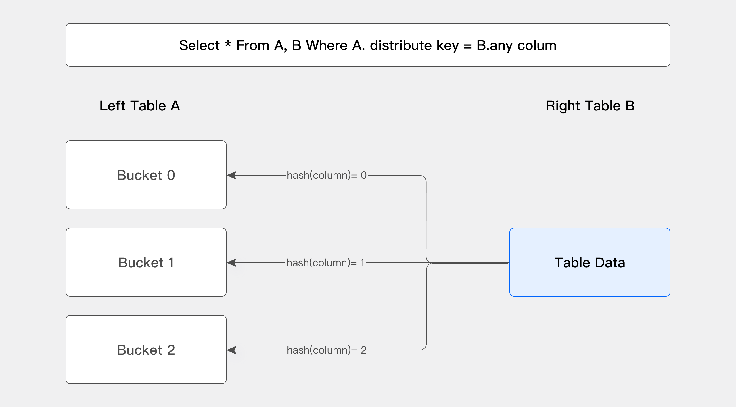
+
上面的图片展示了 Bucket Shuffle Join 的工作原理。SQL 语句为 A 表 join B 表,并且 join 的等值表达式命中了 A 的数据分布列。而 Bucket Shuffle Join 会根据 A 表的数据分布信息,将 B 表的数据发送到对应的 A 表的数据存储计算节点。Bucket Shuffle Join 开销如下:
diff --git a/i18n/zh-CN/docusaurus-plugin-content-docs/current/query/join-optimization/doris-join-optimization.md b/i18n/zh-CN/docusaurus-plugin-content-docs/current/query/join-optimization/doris-join-optimization.md
index 87c6201..6bd7049 100644
--- a/i18n/zh-CN/docusaurus-plugin-content-docs/current/query/join-optimization/doris-join-optimization.md
+++ b/i18n/zh-CN/docusaurus-plugin-content-docs/current/query/join-optimization/doris-join-optimization.md
@@ -48,7 +48,7 @@
它适用的场景是比较通用的,同时能够支持 Hash Join 和 Nest loop Join,它的网络开销 N * T(R)。
- 
+ 
左表数据不移动,右表数据发送到左表数据的扫描节点。
@@ -58,7 +58,8 @@
它的网络开销则是:T(S) + T(R),但它只能支持 Hash Join,因为它是根据 Join 的条件也去做计算分桶的。
- 
+ 
+
左右表数据根据分区,计算的结果发送到不同的分区节点上。
@@ -68,7 +69,7 @@
它的网络开销则是:T(R)相当于只 Shuffle 右表的数据就可以了。
- 
+ 
左表数据不移动,右表数据根据分区计算的结果发送到左表扫表的节点
@@ -76,7 +77,7 @@
它与 Bucket Shuffle Join 相似,相当于在数据导入的时候,根据预设的 Join 列的场景已经做好了数据的 Shuffle。那么实际查询的时候就可以直接进行 Join 计算而不需要考虑数据的 Shuffle 问题了。
- 
+ 
数据已经预先分区,直接在本地进行 Join 计算
@@ -139,7 +140,7 @@
接下来看右图,把 Join 的顺序调整了一下。把 a 表先与 c 表 Join,生成的中间结果只有 100,然后最终再与 b 表 Join 计算。最终的 Join 结果是一样的,但是它生成的中间结果有 20 倍的差距,这就会产生一个很大的性能 Diff 了。
-
+
Doris 目前支持基于规则的 Join Reorder 算法。它的逻辑是:
diff --git a/i18n/zh-CN/docusaurus-plugin-content-docs/current/table-design/best-practice.md b/i18n/zh-CN/docusaurus-plugin-content-docs/current/table-design/best-practice.md
index c8097d0..c1aee06 100644
--- a/i18n/zh-CN/docusaurus-plugin-content-docs/current/table-design/best-practice.md
+++ b/i18n/zh-CN/docusaurus-plugin-content-docs/current/table-design/best-practice.md
@@ -51,7 +51,7 @@
### 01 DUPLICATE KEY 表模型
-
+
只指定排序列,相同的 KEY 行不会合并。
@@ -83,7 +83,7 @@
### 02 AGGREGATE KEY 表模型
-
+
AGGREGATE KEY 相同时,新旧记录进行聚合,目前支持的聚合方式:
@@ -395,7 +395,7 @@
## 4 数据表创建
-
+
建表时除了要注意数据表模型、索引和字段类型的选择还需要注意分区分桶的设置。
diff --git a/i18n/zh-CN/docusaurus-plugin-content-docs/current/table-design/index/bitmap-index.md b/i18n/zh-CN/docusaurus-plugin-content-docs/current/table-design/index/bitmap-index.md
index 318fffd..afeb86c 100644
--- a/i18n/zh-CN/docusaurus-plugin-content-docs/current/table-design/index/bitmap-index.md
+++ b/i18n/zh-CN/docusaurus-plugin-content-docs/current/table-design/index/bitmap-index.md
@@ -29,7 +29,7 @@
如下图,bitmap 索引将每个被索引的列的值作为 KEY,使用每个 BIT 表示一行,当这行中包含这个值时,设置为 1,否则设置为 0。
-
+
## 适用场景
diff --git a/i18n/zh-CN/docusaurus-plugin-content-docs/current/table-design/index/bloomfilter.md b/i18n/zh-CN/docusaurus-plugin-content-docs/current/table-design/index/bloomfilter.md
index ee6a8c3..e6e59c1 100644
--- a/i18n/zh-CN/docusaurus-plugin-content-docs/current/table-design/index/bloomfilter.md
+++ b/i18n/zh-CN/docusaurus-plugin-content-docs/current/table-design/index/bloomfilter.md
@@ -40,7 +40,7 @@
下图所示出一个 m=18, k=3(m 是该 Bit 数组的大小,k 是 Hash 函数的个数)的 Bloom Filter 示例。集合中的 x、y、z 三个元素通过 3 个不同的哈希函数散列到位数组中。当查询元素 w 时,通过 Hash 函数计算之后因为有一个比特为 0,因此 w 不在该集合中。
-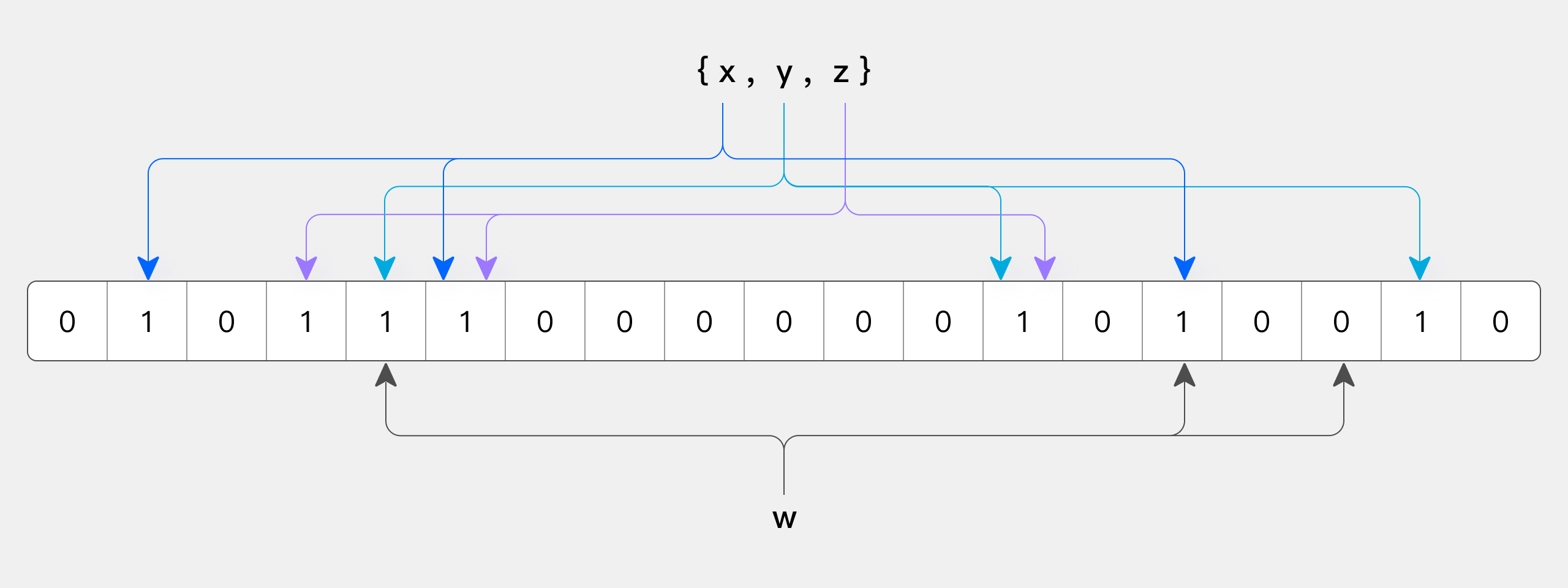
+
同样是如果某个元素经过哈希函数计算后得到所有的偏移位置,若这些位置全都为 1,则判断这个元素在这个集合中。
diff --git a/i18n/zh-CN/docusaurus-plugin-content-docs/version-1.2/query-acceleration/join-optimization/doris-join-optimization.md b/i18n/zh-CN/docusaurus-plugin-content-docs/version-1.2/query-acceleration/join-optimization/doris-join-optimization.md
index 98ad05f..8d9e43e 100644
--- a/i18n/zh-CN/docusaurus-plugin-content-docs/version-1.2/query-acceleration/join-optimization/doris-join-optimization.md
+++ b/i18n/zh-CN/docusaurus-plugin-content-docs/version-1.2/query-acceleration/join-optimization/doris-join-optimization.md
@@ -33,7 +33,7 @@
- Hash Join:在右表上根据等值 Join 列建立哈希表,左表流式的利用哈希表进行 Join 计算,它的限制是只能适用于等值 Join。
- Nest Loop Join:通过两个 for 循环,很直观。然后它适用的场景就是不等值的 Join,例如:大于小于或者是需要求笛卡尔积的场景。它是一个通用的 Join 算子,但是性能表现差。
-作为分布式的 MPP 数据库, 在 Join 的过程中是需要进行数据的 Shuffle。数据需要进行拆分调度,才能保证最终的 Join 结果是正确的。举个简单的例子,假设关系S 和 R 进行Join,N 表示参与 Join 计算的节点的数量;T 则表示关系的 Tuple 数目。
+作为分布式的 MPP 数据库,在 Join 的过程中是需要进行数据的 Shuffle。数据需要进行拆分调度,才能保证最终的 Join 结果是正确的。举个简单的例子,假设关系 S 和 R 进行 Join,N 表示参与 Join 计算的节点的数量;T 则表示关系的 Tuple 数目。
@@ -47,7 +47,7 @@
它适用的场景是比较通用的,同时能够支持 Hash Join 和 Nest loop Join,它的网络开销 N * T(R)。
- 
+ 
左表数据不移动,右表数据发送到左表数据的扫描节点。
@@ -57,7 +57,7 @@
它的网络开销则是:T(R) + T(N),但它只能支持 Hash Join,因为它是根据 Join 的条件也去做计算分桶的。
- 
+ 
左右表数据根据分区,计算的结果发送到不同的分区节点上。
@@ -67,7 +67,7 @@
它的网络开销则是:T(R)相当于只 Shuffle 右表的数据就可以了。
- 
+ 
左表数据不移动,右表数据根据分区计算的结果发送到左表扫表的节点
@@ -75,20 +75,20 @@
它与 Bucket Shuffle Join 相似,相当于在数据导入的时候,根据预设的 Join 列的场景已经做好了数据的 Shuffle。那么实际查询的时候就可以直接进行 Join 计算而不需要考虑数据的 Shuffle 问题了。
- 
+ 
数据已经预先分区,直接在本地进行 Join 计算
### 四种 Shuffle 方式对比
-| Shuffle方式 | 网络开销 | 物理算子 | 适用场景 |
+| Shuffle 方式 | 网络开销 | 物理算子 | 适用场景 |
| -------------- | ----------- | -------------------------- | ------------------------------------------------------------ |
| BroadCast | N * T(R) | Hash Join / Nest Loop Join | 通用 |
| Shuffle | T(S) + T(R) | Hash Join | 通用 |
-| Bucket Shuffle | T(R) | Hash Join | Join条件中存在左表的分布式列,且左表执行时为单分区 |
-| Colocate | 0 | Hash Join | Join条件中存在左表的分布式列,且左右表同属于一个Colocate Group |
+| Bucket Shuffle | T(R) | Hash Join | Join 条件中存在左表的分布式列,且左表执行时为单分区 |
+| Colocate | 0 | Hash Join | Join 条件中存在左表的分布式列,且左右表同属于一个 Colocate Group |
-N : 参与 Join 计算的 Instance 个数
+N:参与 Join 计算的 Instance 个数
T(关系) : 关系的 Tuple 数目
@@ -108,20 +108,20 @@
Runtime Filter 适用的场景有两个要求:
-- 第一个要求就是左表大右表小,因为构建 Runtime Filter是需要承担计算成本的,包括一些内存的开销。
+- 第一个要求就是左表大右表小,因为构建 Runtime Filter 是需要承担计算成本的,包括一些内存的开销。
- 第二个要求就是左右表 Join 出来的结果很少,说明这个 Join 可以过滤掉左表的绝大部分数据。
当符合上面两个条件的情况下,开启 Runtime Filter 就能收获比较好的效果
当 Join 列为左表的 Key 列时,RuntimeFilter 会下推到存储引擎。Doris 本身支持延迟物化,
-延迟物化简单来说是这样的:假如需要扫描 A、B、C 三列,在 A 列上有一个过滤条件: A 等于 2,要扫描 100 行的话,可以先把 A 列的 100 行扫描出来,再通过 A = 2 这个过滤条件过滤。之后通过过滤完成后的结果,再去读取 B、C 列,这样就能极大的降低数据的读取 IO。所以说 Runtime Filter 如果在 Key 列上生成,同时利用 Doris 本身的延迟物化来进一步提升查询的性能。
+延迟物化简单来说是这样的:假如需要扫描 A、B、C 三列,在 A 列上有一个过滤条件:A 等于 2,要扫描 100 行的话,可以先把 A 列的 100 行扫描出来,再通过 A = 2 这个过滤条件过滤。之后通过过滤完成后的结果,再去读取 B、C 列,这样就能极大的降低数据的读取 IO。所以说 Runtime Filter 如果在 Key 列上生成,同时利用 Doris 本身的延迟物化来进一步提升查询的性能。
### Runtime Filter 类型
Doris 提供了三种不同的 Runtime Filter 类型:
-- **IN** 的优点是过滤效果明显,且快速。它的缺点首先第一个它只适用于 BroadCast,第二,它右表超过一定数据量的时候就失效了,当前 Doris 目前配置的是1024,即右表如果大于 1024,IN 的 Runtime Filter 就直接失效了。
+- **IN** 的优点是过滤效果明显,且快速。它的缺点首先第一个它只适用于 BroadCast,第二,它右表超过一定数据量的时候就失效了,当前 Doris 目前配置的是 1024,即右表如果大于 1024,IN 的 Runtime Filter 就直接失效了。
- **MinMax** 的优点是开销比较小。它的缺点就是对数值列还有比较好的效果,但对于非数值列,基本上就没什么效果。
- **Bloom Filter** 的特点就是通用,适用于各种类型、效果也比较好。缺点就是它的配置比较复杂并且计算较高。
@@ -133,7 +133,7 @@
接下来看右图,把 Join 的顺序调整了一下。把 a 表先与 c 表 Join,生成的中间结果只有 100,然后最终再与 b 表 Join 计算。最终的 Join 结果是一样的,但是它生成的中间结果有 20 倍的差距,这就会产生一个很大的性能 Diff 了。
-
+
Doris 目前支持基于规则的 Join Reorder 算法。它的逻辑是:
@@ -162,7 +162,7 @@

-进一步分析 Profile 之后,发现 BuildRows,就是右表的数据量是大概 2500 万。而 ProbeRows ( ProbeRows 是左表的数据量)只有 1 万多。这种场景下右表是远远大于左表,这显然是个不合理的情况。这显然说明 Join 的顺序出现了一些问题。这时候尝试改变 Session 变量,开启 Join Reorder。
+进一步分析 Profile 之后,发现 BuildRows,就是右表的数据量是大概 2500 万。而 ProbeRows(ProbeRows 是左表的数据量)只有 1 万多。这种场景下右表是远远大于左表,这显然是个不合理的情况。这显然说明 Join 的顺序出现了一些问题。这时候尝试改变 Session 变量,开启 Join Reorder。
```
set enable_cost_based_join_reorder = true
@@ -176,7 +176,7 @@
### 案例二
-存在一个慢查询,查看 Profile 之后,整个 Join 节点耗时大概44秒。它的右表有 1000 万,左表有 6000 万,最终返回的结果也只有 6000 万。
+存在一个慢查询,查看 Profile 之后,整个 Join 节点耗时大概 44 秒。它的右表有 1000 万,左表有 6000 万,最终返回的结果也只有 6000 万。

@@ -184,13 +184,13 @@

-当右表超过1024行的话, IN 是不生效的,所以根本起不到什么过滤的效果,所以尝试调整 RuntimeFilter 的类型。
+当右表超过 1024 行的话,IN 是不生效的,所以根本起不到什么过滤的效果,所以尝试调整 RuntimeFilter 的类型。
这里改为了 BloomFilter,左表的 6000 万条数据过滤了 5900 万条。基本上 99% 的数据都被过滤掉了,这个效果是很显著的。查询也从原来的 44 秒降到了 13 秒,性能提升了大概也是三倍多。
### 案例三
-下面是一个比较极端的 Case,通过一些环境变量调优也没有办法解决,因为它涉及到 SQL Rewrite,所以这里列出来了原始的 SQL 。
+下面是一个比较极端的 Case,通过一些环境变量调优也没有办法解决,因为它涉及到 SQL Rewrite,所以这里列出来了原始的 SQL。
```sql
select 100.00 * sum (case
@@ -205,13 +205,13 @@
and 1 shipdate < date '1997-06-01' + interval '1' month
```
-这个 Join 查询是很简单的,单纯的一个左右表的 Join 。当然它上面有一些过滤条件,打开 Profile 的时候,发现整个查询 Hash Join 执行了三分多钟,它是一个 BroadCast 的 Join,它的右表有 2 亿条,左表只有 70 万。在这种情况下选择了 Broadcast Join 是不合理的,这相当于要把 2 亿条做一个 Hash Table,然后用 70 万条遍历两亿条的 Hash Table ,这显然是不合理的。
+这个 Join 查询是很简单的,单纯的一个左右表的 Join。当然它上面有一些过滤条件,打开 Profile 的时候,发现整个查询 Hash Join 执行了三分多钟,它是一个 BroadCast 的 Join,它的右表有 2 亿条,左表只有 70 万。在这种情况下选择了 Broadcast Join 是不合理的,这相当于要把 2 亿条做一个 Hash Table,然后用 70 万条遍历两亿条的 Hash Table,这显然是不合理的。

-为什么会产生不合理的 Join 顺序呢?其实这个左表是一个 10 亿条级别的大表,它上面加了两个过滤条件,加完这两个过滤条件之后, 10 亿条的数据就剩 70 万条了。但 Doris 目前没有一个好的统计信息收集的框架,所以它不知道这个过滤条件的过滤率到底怎么样。所以这个 Join 顺序安排的时候,就选择了错误的 Join 的左右表顺序,导致它的性能是极其低下的。
+为什么会产生不合理的 Join 顺序呢?其实这个左表是一个 10 亿条级别的大表,它上面加了两个过滤条件,加完这两个过滤条件之后,10 亿条的数据就剩 70 万条了。但 Doris 目前没有一个好的统计信息收集的框架,所以它不知道这个过滤条件的过滤率到底怎么样。所以这个 Join 顺序安排的时候,就选择了错误的 Join 的左右表顺序,导致它的性能是极其低下的。
-下图是改写完成之后的一个 SQL 语句,在 Join 后面添加了一个Join Hint,在Join 后面加一个方括号,然后把需要的 Join 方式写入。这里选择了 Shuffle Join,可以看到右边它实际查询计划里面看到这个数据确实是做了 Partition ,原先 3 分钟的耗时通过这样的改写完之后只剩下 7 秒,性能提升明显
+下图是改写完成之后的一个 SQL 语句,在 Join 后面添加了一个 Join Hint,在 Join 后面加一个方括号,然后把需要的 Join 方式写入。这里选择了 Shuffle Join,可以看到右边它实际查询计划里面看到这个数据确实是做了 Partition,原先 3 分钟的耗时通过这样的改写完之后只剩下 7 秒,性能提升明显

@@ -220,7 +220,7 @@
最后我们总结 Doris Join 优化调优的四点建议:
- 第一点:在做 Join 的时候,要尽量选择同类型或者简单类型的列,同类型的话就减少它的数据 Cast,简单类型本身 Join 计算就很快。
-- 第二点:尽量选择 Key 列进行 Join, 原因前面在 Runtime Filter 的时候也介绍了,Key 列在延迟物化上能起到一个比较好的效果。
-- 第三点:大表之间的 Join ,尽量让它 Colocation ,因为大表之间的网络开销是很大的,如果需要去做 Shuffle 的话,代价是很高的。
+- 第二点:尽量选择 Key 列进行 Join,原因前面在 Runtime Filter 的时候也介绍了,Key 列在延迟物化上能起到一个比较好的效果。
+- 第三点:大表之间的 Join,尽量让它 Colocation,因为大表之间的网络开销是很大的,如果需要去做 Shuffle 的话,代价是很高的。
- 第四点:合理的使用 Runtime Filter,它在 Join 过滤率高的场景下效果是非常显著的。但是它并不是万灵药,而是有一定副作用的,所以需要根据具体的 SQL 的粒度做开关。
- 最后:要涉及到多表 Join 的时候,需要去判断 Join 的合理性。尽量保证左表为大表,右表为小表,然后 Hash Join 会优于 Nest Loop Join。必要的时可以通过 SQL Rewrite,利用 Hint 去调整 Join 的顺序。
diff --git a/i18n/zh-CN/docusaurus-plugin-content-docs/version-2.0.json b/i18n/zh-CN/docusaurus-plugin-content-docs/version-2.0.json
index 7976c05..c92513a 100644
--- a/i18n/zh-CN/docusaurus-plugin-content-docs/version-2.0.json
+++ b/i18n/zh-CN/docusaurus-plugin-content-docs/version-2.0.json
@@ -67,7 +67,7 @@
     "message": "数据湖分析",
     "description": "The label for category Data Lake Analytics in sidebar docs"
   },
-  "sidebar.docs.category.Analyzing Databas": {
+  "sidebar.docs.category.Analyzing Database": {
     "message": "数据库分析",
     "description": "The label for category Database Analytics.Multi Catalog in sidebar docs"
   },
@@ -143,7 +143,7 @@
     "message": "集群管理",
     "description": "The label for category cluster management in sidebar docs"
   },
-  "sidebar.docs.category.Manging Data": {
+  "sidebar.docs.category.Managing Data": {
     "message": "数据管理",
     "description": "The label for category Manging Data in sidebar docs"
   },
diff --git a/i18n/zh-CN/docusaurus-plugin-content-docs/version-2.0/admin-manual/data-admin/ccr.md b/i18n/zh-CN/docusaurus-plugin-content-docs/version-2.0/admin-manual/data-admin/ccr.md
index 38cd422..d98c74a 100644
--- a/i18n/zh-CN/docusaurus-plugin-content-docs/version-2.0/admin-manual/data-admin/ccr.md
+++ b/i18n/zh-CN/docusaurus-plugin-content-docs/version-2.0/admin-manual/data-admin/ccr.md
@@ -53,7 +53,7 @@
### 架构说明
-
+
CCR 工具主要依赖一个轻量级进程:Syncers。Syncers 会从源集群获取 binlog,直接将元数据应用于目标集群,通知目标集群从源集群拉取数据。从而实现全量和增量迁移。
diff --git a/i18n/zh-CN/docusaurus-plugin-content-docs/version-2.0/data-operate/import/routine-load-manual.md b/i18n/zh-CN/docusaurus-plugin-content-docs/version-2.0/data-operate/import/routine-load-manual.md
index 7932beb..905dc61 100644
--- a/i18n/zh-CN/docusaurus-plugin-content-docs/version-2.0/data-operate/import/routine-load-manual.md
+++ b/i18n/zh-CN/docusaurus-plugin-content-docs/version-2.0/data-operate/import/routine-load-manual.md
@@ -62,7 +62,7 @@
Routine Load 的导入具体流程如下图展示:
-
+
1. Client 向 FE 提交 Routine Load 常驻 Routine Load Job
diff --git a/i18n/zh-CN/docusaurus-plugin-content-docs/version-2.0/get-starting/what-is-apache-doris.md b/i18n/zh-CN/docusaurus-plugin-content-docs/version-2.0/get-starting/what-is-apache-doris.md
index b4aba64..c61667c 100644
--- a/i18n/zh-CN/docusaurus-plugin-content-docs/version-2.0/get-starting/what-is-apache-doris.md
+++ b/i18n/zh-CN/docusaurus-plugin-content-docs/version-2.0/get-starting/what-is-apache-doris.md
@@ -36,7 +36,7 @@
如下图所示,数据源经过各种数据集成和加工处理后,通常会入库到实时数据仓库 Apache Doris 和离线湖仓(Hive, Iceberg, Hudi 中),Apache Doris 被广泛应用在以下场景中。
-
+
- 报表分析
@@ -63,7 +63,7 @@
这两类进程都是可以横向扩展的,单集群可以支持到数百台机器,数十 PB 的存储容量。并且这两类进程通过一致性协议来保证服务的高可用和数据的高可靠。这种高度集成的架构设计极大的降低了一款分布式系统的运维成本。
-
+
### 使用接口
@@ -97,12 +97,12 @@
在**查询引擎**方面,Doris 采用 MPP 的模型,节点间和节点内都并行执行,也支持多个大表的分布式 Shuffle Join,从而能够更好应对复杂查询。
-
+
**Doris 查询引擎是向量化**的查询引擎,所有的内存结构能够按照列式布局,能够达到大幅减少虚函数调用、提升 Cache 命中率,高效利用 SIMD 指令的效果。在宽表聚合场景下性能是非向量化引擎的 5-10 倍。
-
+
**Doris 采用了 Adaptive Query Execution 技术,** 可以根据 Runtime Statistics 来动态调整执行计划,比如通过 Runtime Filter 技术能够在运行时生成 Filter 推到 Probe 侧,并且能够将 Filter 自动穿透到 Probe 侧最底层的 Scan 节点,从而大幅减少 Probe 的数据量,加速 Join 性能。Doris 的 Runtime Filter 支持 In/Min/Max/Bloom Filter。
diff --git a/i18n/zh-CN/docusaurus-plugin-content-docs/version-2.0/lakehouse/lakehouse-overview.md b/i18n/zh-CN/docusaurus-plugin-content-docs/version-2.0/lakehouse/lakehouse-overview.md
index f6452ef..ee6202d 100644
--- a/i18n/zh-CN/docusaurus-plugin-content-docs/version-2.0/lakehouse/lakehouse-overview.md
+++ b/i18n/zh-CN/docusaurus-plugin-content-docs/version-2.0/lakehouse/lakehouse-overview.md
@@ -1,11 +1,11 @@
---
{
"title": "湖仓一体概述",
- "language": "zh-CN"
+ "language": "en"
}
---
-<!--
+<!--
Licensed to the Apache Software Foundation (ASF) under one
or more contributor license agreements. See the NOTICE file
distributed with this work for additional information
@@ -24,7 +24,6 @@
under the License.
-->
-
湖仓一体之前,数据分析经历了数据库、数据仓库和数据湖分析三个时代。
- 首先是数据库,它是一个最基础的概念,主要负责联机事务处理,也提供基本的数据分析能力。
@@ -52,7 +51,7 @@
Doris 通过多源数据目录(Multi-Catalog)功能,支持了包括 Apache Hive、Apache Iceberg、Apache Hudi、Apache Paimon(Incubating)、Elasticsearch、MySQL、Oracle、SQLSserver 等主流数据湖、数据库的连接访问。以及可以通过 Apache Ranger 等进行统一的权限管理,具体架构如下:
-
+
其数据湖的主要对接流程为:
@@ -77,7 +76,7 @@
- 数据读取:通过 NativeReader 可以高效的读取存放在 HDFS、对象存储上的 Parquet、ORC、Text 格式数据。也可以通过 JniConnector 对接 Java 大数据生态。
-
+
### 高效缓存策略
@@ -87,7 +86,7 @@
Doris 提供了手动同步元数据、定期自动同步元数据、元数据订阅(只支持 HiveMetastore)三种方式来同步数据湖的元数据信息到 Doris,并将元数据存储在 Doris 的 FE 的内存中。当用户发起查询后 Doris 直接从内存中获取元数据并快速生成查询规划。保障了元数据的实时和高效。在元数据同步上 Doris 通过并发的元数据事件合并实现高效的元数据同步,其每秒可以处理 100 个以上的元数据事件。
-
+
**高效的数据缓存**
@@ -97,7 +96,7 @@
- 缓存淘汰(更新)策略:同时当 Doris 发现数据文件对应的元数据更新后,会及时淘汰缓存以保障数据的一致性。
-
+
**查询结果缓存和分区缓存**
@@ -106,7 +105,7 @@
- 分区缓存:Doris 还支持将部分分区数据缓存在 BE 端提升查询效率。比如查询最近 7 天的数据,可以将前 6 天的计算后的缓存结果,和当天的事实计算结果进行合并,得到最终查询结果,最大限度减少实时计算的数据量,提升查询效率。
-
+
### 高效的 Native Reader
@@ -118,7 +117,7 @@
- 向量化读取数据:同时在文件数据的读取过程中我们引入向量化的方式读取数据,极大加速了数据读取效率。
-
+
### Merge IO
@@ -128,7 +127,7 @@
Merge IO 的确定是它可能会读取一些不必要的数据,因为它把中间可能不必要读取的数据合并起来一块读过来了。但是从整体的吞吐上来讲其性能有很大的提高,在碎文件(比如:1KB - 1MB)较多的场景优化效果很明显。同时我们通过控制 Merge IO 的大小来达到整体的平衡。
-
+
### 统计信息提高查询规划效果
@@ -140,7 +139,7 @@
在一些场景下用户历史数据可能很少查找,但是热数据会被经常访问,因此我们也提供了基于分区的统计信息收集在保障热数据高效的查询效率和统计信息收集对 BE 产生负载的中间取得平衡。
-
+
## 多源数据目录
@@ -172,13 +171,13 @@
- External Catalog
- 可以通过 [CREATE CATALOG](../sql-manual/sql-reference/Data-Definition-Statements/Create/CREATE-CATALOG) 命令创建一个 External Catalog。创建后,可以通过 [SHOW CATALOGS](../sql-manual/sql-reference/Show-Statements/SHOW-CATALOGS) 命令查看已创建的 Catalog。
+ 可以通过 [CREATE CATALOG](../sql-manual/sql-statements/Data-Definition-Statements/Create/CREATE-CATALOG) 命令创建一个 External Catalog。创建后,可以通过 [SHOW CATALOGS](../sql-manual/sql-statements/Show-Statements/SHOW-CATALOGS) 命令查看已创建的 Catalog。
- 切换 Catalog
用户登录 Doris 后,默认进入 Internal Catalog,因此默认的使用和之前版本并无差别,可以直接使用 `SHOW DATABASES`,`USE DB` 等命令查看和切换数据库。
- 用户可以通过 [SWITCH](../sql-manual/sql-reference/Utility-Statements/SWITCH) 命令切换 Catalog。如:
+ 用户可以通过 [SWITCH](../sql-manual/sql-statements/Utility-Statements/SWITCH) 命令切换 Catalog。如:
```Plain
SWITCH internal;
@@ -189,7 +188,7 @@
- 删除 Catalog
- 可以通过 [DROP CATALOG](../sql-manual/sql-reference/Data-Definition-Statements/Drop/DROP-CATALOG) 命令删除一个 External Catalog,Internal Catalog 无法删除。该操作仅会删除 Doris 中该 Catalog 的映射信息,并不会修改或变更任何外部数据目录的内容。
+ 可以通过 [DROP CATALOG](../sql-manual/sql-statements/Data-Definition-Statements/Drop/DROP-CATALOG) 命令删除一个 External Catalog,Internal Catalog 无法删除。该操作仅会删除 Doris 中该 Catalog 的映射信息,并不会修改或变更任何外部数据目录的内容。
### 连接示例
@@ -197,7 +196,7 @@
这里我们通过连接一个 Hive 集群说明如何使用 Catalog 功能。
-更多关于 Hive 的说明,请参阅:[Hive Catalog](../lakehouse/datalake/hive)
+更多关于 Hive 的说明,请参阅:[Hive Catalog](../lakehouse/datalake-analytics/hive)
**1. 创建 Catalog**
@@ -208,7 +207,7 @@
);
```
-更多查看:[CREATE CATALOG 语法帮助](../sql-manual/sql-reference/Data-Definition-Statements/Create/CREATE-CATALOG)
+更多查看:[CREATE CATALOG 语法帮助](../sql-manual/sql-statements/Data-Definition-Statements/Create/CREATE-CATALOG)
**2. 查看 Catalog**
@@ -224,11 +223,11 @@
+-----------+-------------+----------+-----------+-------------------------+---------------------+------------------------+
```
-- [SHOW CATALOGS 语法帮助](../sql-manual/sql-reference/Show-Statements/SHOW-CATALOGS)
+- [SHOW CATALOGS 语法帮助](../sql-manual/sql-statements/Show-Statements/SHOW-CATALOGS)
-- 可以通过 [SHOW CREATE CATALOG](../sql-manual/sql-reference/Show-Statements/SHOW-CREATE-CATALOG) 查看创建 Catalog 的语句。
+- 可以通过 [SHOW CREATE CATALOG](../sql-manual/sql-statements/Show-Statements/SHOW-CREATE-CATALOG) 查看创建 Catalog 的语句。
-- 可以通过 [ALTER CATALOG](../sql-manual/sql-reference/Data-Definition-Statements/Alter/ALTER-CATALOG) 修改 Catalog 的属性。
+- 可以通过 [ALTER CATALOG](../sql-manual/sql-statements/Data-Definition-Statements/Alter/ALTER-CATALOG) 修改 Catalog 的属性。
**4. 切换 Catalog**
@@ -251,7 +250,7 @@
+-----------+
```
-查看更多:[SWITCH 语法帮助](../sql-manual/sql-reference/Utility-Statements/SWITCH)
+查看更多:[SWITCH 语法帮助](../sql-manual/sql-statements/Utility-Statements/SWITCH)
**5. 使用 Catalog**
@@ -387,15 +386,15 @@
使用 Doris 对 External Catalog 中库表进行访问时,默认情况下,依赖 Doris 自身的权限访问管理功能。
-Doris 的权限管理功能提供了对 Catalog 层级的扩展,具体可参阅 [权限管理](../admin-manual/privilege-ldap/user-privilege) 文档。
+Doris 的权限管理功能提供了对 Catalog 层级的扩展,具体可参阅 [认证和鉴权](../admin-manual/auth/authentication-and-authorization.md) 文档。
用户也可以通过 `access_controller.class` 属性指定自定义的鉴权类。如通过指定:
```
-"access_controller.class" = "org.apache.doris.catalog.authorizer.RangerHiveAccessControllerFactory"
+"access_controller.class" = "org.apache.doris.catalog.authorizer.ranger.hive.RangerHiveAccessControllerFactory"
```
-则可以使用 Apache Range 对 Hive Catalog 进行鉴权管理。详细信息请参阅:[Hive Catalog](../lakehouse/datalake/hive)
+则可以使用 Apache Range 对 Hive Catalog 进行鉴权管理。详细信息请参阅:[Hive Catalog](../lakehouse/datalake-analytics/hive)
### 指定需要同步的数据库
@@ -408,7 +407,7 @@
:::tip
- 当 `include_database_list` 和 `exclude_database_list` 有重合的 database 配置时,`exclude_database_list`会优先生效。
-- 连接 JDBC 时,上述 2 个配置需要和配置 `only_specified_database` 搭配使用,详见 [JDBC](../lakehouse/database/jdbc)
+- 连接 JDBC 时,上述 2 个配置需要和配置 `only_specified_database` 搭配使用,详见 [JDBC](../lakehouse/database/jdbc.md)
:::
### 元数据更新
@@ -417,11 +416,11 @@
用户可以通过以下几种方式刷新元数据。
-#### 手动刷新
+**手动刷新**
-用户需要通过 [REFRESH](../sql-manual/sql-reference/Utility-Statements/REFRESH) 命令手动刷新元数据。
+用户需要通过 [REFRESH](../sql-manual/sql-statements/Utility-Statements/REFRESH) 命令手动刷新元数据。
-#### 定时刷新
+**定时刷新**
在创建 catalog 时,在 properties 中指定刷新时间参数`metadata_refresh_interval_sec` ,以秒为单位,若在创建 catalog 时设置了该参数,FE 的 master 节点会根据参数值定时刷新该 catalog。目前支持三种类型
@@ -440,6 +439,6 @@
);
```
-#### 自动刷新
+**自动刷新**
-自动刷新目前仅支持 [Hive Catalog](../lakehouse/datalake/hive)。
\ No newline at end of file
+自动刷新目前仅支持 [Hive Catalog](../lakehouse/datalake-analytics/hive)。
diff --git a/i18n/zh-CN/docusaurus-plugin-content-docs/version-2.0/query/join-optimization/bucket-shuffle-join.md b/i18n/zh-CN/docusaurus-plugin-content-docs/version-2.0/query/join-optimization/bucket-shuffle-join.md
index 301723c..e028736 100644
--- a/i18n/zh-CN/docusaurus-plugin-content-docs/version-2.0/query/join-optimization/bucket-shuffle-join.md
+++ b/i18n/zh-CN/docusaurus-plugin-content-docs/version-2.0/query/join-optimization/bucket-shuffle-join.md
@@ -48,7 +48,7 @@
在 FE 之中保存了 Doris 每个表的数据分布信息,如果 join 语句命中了表的数据分布列,我们应该使用数据分布信息来减少 join 语句的网络与内存开销,这就是 Bucket Shuffle Join 的思路来源。
-
+
上面的图片展示了 Bucket Shuffle Join 的工作原理。SQL 语句为 A 表 join B 表,并且 join 的等值表达式命中了 A 的数据分布列。而 Bucket Shuffle Join 会根据 A 表的数据分布信息,将 B 表的数据发送到对应的 A 表的数据存储计算节点。Bucket Shuffle Join 开销如下:
diff --git a/i18n/zh-CN/docusaurus-plugin-content-docs/version-2.0/query/join-optimization/doris-join-optimization.md b/i18n/zh-CN/docusaurus-plugin-content-docs/version-2.0/query/join-optimization/doris-join-optimization.md
index 87c6201..581887c 100644
--- a/i18n/zh-CN/docusaurus-plugin-content-docs/version-2.0/query/join-optimization/doris-join-optimization.md
+++ b/i18n/zh-CN/docusaurus-plugin-content-docs/version-2.0/query/join-optimization/doris-join-optimization.md
@@ -48,7 +48,7 @@
它适用的场景是比较通用的,同时能够支持 Hash Join 和 Nest loop Join,它的网络开销 N * T(R)。
- 
+ 
左表数据不移动,右表数据发送到左表数据的扫描节点。
@@ -58,7 +58,7 @@
它的网络开销则是:T(S) + T(R),但它只能支持 Hash Join,因为它是根据 Join 的条件也去做计算分桶的。
- 
+ 
左右表数据根据分区,计算的结果发送到不同的分区节点上。
@@ -68,7 +68,7 @@
它的网络开销则是:T(R)相当于只 Shuffle 右表的数据就可以了。
- 
+ 
左表数据不移动,右表数据根据分区计算的结果发送到左表扫表的节点
@@ -76,7 +76,7 @@
它与 Bucket Shuffle Join 相似,相当于在数据导入的时候,根据预设的 Join 列的场景已经做好了数据的 Shuffle。那么实际查询的时候就可以直接进行 Join 计算而不需要考虑数据的 Shuffle 问题了。
- 
+ 
数据已经预先分区,直接在本地进行 Join 计算
@@ -139,7 +139,7 @@
接下来看右图,把 Join 的顺序调整了一下。把 a 表先与 c 表 Join,生成的中间结果只有 100,然后最终再与 b 表 Join 计算。最终的 Join 结果是一样的,但是它生成的中间结果有 20 倍的差距,这就会产生一个很大的性能 Diff 了。
-
+
Doris 目前支持基于规则的 Join Reorder 算法。它的逻辑是:
diff --git a/i18n/zh-CN/docusaurus-plugin-content-docs/version-2.0/table-design/best-practice.md b/i18n/zh-CN/docusaurus-plugin-content-docs/version-2.0/table-design/best-practice.md
index c8097d0..c1aee06 100644
--- a/i18n/zh-CN/docusaurus-plugin-content-docs/version-2.0/table-design/best-practice.md
+++ b/i18n/zh-CN/docusaurus-plugin-content-docs/version-2.0/table-design/best-practice.md
@@ -51,7 +51,7 @@
### 01 DUPLICATE KEY 表模型
-
+
只指定排序列,相同的 KEY 行不会合并。
@@ -83,7 +83,7 @@
### 02 AGGREGATE KEY 表模型
-
+
AGGREGATE KEY 相同时,新旧记录进行聚合,目前支持的聚合方式:
@@ -395,7 +395,7 @@
## 4 数据表创建
-
+
建表时除了要注意数据表模型、索引和字段类型的选择还需要注意分区分桶的设置。
diff --git a/i18n/zh-CN/docusaurus-plugin-content-docs/version-2.0/table-design/index/bitmap-index.md b/i18n/zh-CN/docusaurus-plugin-content-docs/version-2.0/table-design/index/bitmap-index.md
index 318fffd..afeb86c 100644
--- a/i18n/zh-CN/docusaurus-plugin-content-docs/version-2.0/table-design/index/bitmap-index.md
+++ b/i18n/zh-CN/docusaurus-plugin-content-docs/version-2.0/table-design/index/bitmap-index.md
@@ -29,7 +29,7 @@
如下图,bitmap 索引将每个被索引的列的值作为 KEY,使用每个 BIT 表示一行,当这行中包含这个值时,设置为 1,否则设置为 0。
-
+
## 适用场景
diff --git a/i18n/zh-CN/docusaurus-plugin-content-docs/version-2.0/table-design/index/bloomfilter.md b/i18n/zh-CN/docusaurus-plugin-content-docs/version-2.0/table-design/index/bloomfilter.md
index ee6a8c3..e6e59c1 100644
--- a/i18n/zh-CN/docusaurus-plugin-content-docs/version-2.0/table-design/index/bloomfilter.md
+++ b/i18n/zh-CN/docusaurus-plugin-content-docs/version-2.0/table-design/index/bloomfilter.md
@@ -40,7 +40,7 @@
下图所示出一个 m=18, k=3(m 是该 Bit 数组的大小,k 是 Hash 函数的个数)的 Bloom Filter 示例。集合中的 x、y、z 三个元素通过 3 个不同的哈希函数散列到位数组中。当查询元素 w 时,通过 Hash 函数计算之后因为有一个比特为 0,因此 w 不在该集合中。
-
+
同样是如果某个元素经过哈希函数计算后得到所有的偏移位置,若这些位置全都为 1,则判断这个元素在这个集合中。
diff --git a/i18n/zh-CN/docusaurus-plugin-content-docs/version-2.1/admin-manual/data-admin/ccr.md b/i18n/zh-CN/docusaurus-plugin-content-docs/version-2.1/admin-manual/data-admin/ccr.md
index 38cd422..d98c74a 100644
--- a/i18n/zh-CN/docusaurus-plugin-content-docs/version-2.1/admin-manual/data-admin/ccr.md
+++ b/i18n/zh-CN/docusaurus-plugin-content-docs/version-2.1/admin-manual/data-admin/ccr.md
@@ -53,7 +53,7 @@
### 架构说明
-
+
CCR 工具主要依赖一个轻量级进程:Syncers。Syncers 会从源集群获取 binlog,直接将元数据应用于目标集群,通知目标集群从源集群拉取数据。从而实现全量和增量迁移。
diff --git a/i18n/zh-CN/docusaurus-plugin-content-docs/version-2.1/data-operate/import/routine-load-manual.md b/i18n/zh-CN/docusaurus-plugin-content-docs/version-2.1/data-operate/import/routine-load-manual.md
index f5edc6b..0fbba78 100644
--- a/i18n/zh-CN/docusaurus-plugin-content-docs/version-2.1/data-operate/import/routine-load-manual.md
+++ b/i18n/zh-CN/docusaurus-plugin-content-docs/version-2.1/data-operate/import/routine-load-manual.md
@@ -62,7 +62,7 @@
Routine Load 的导入具体流程如下图展示:
-
+
1. Client 向 FE 提交 Routine Load 常驻 Routine Load Job
diff --git a/i18n/zh-CN/docusaurus-plugin-content-docs/version-2.1/get-starting/what-is-apache-doris.md b/i18n/zh-CN/docusaurus-plugin-content-docs/version-2.1/get-starting/what-is-apache-doris.md
index b4aba64..c61667c 100644
--- a/i18n/zh-CN/docusaurus-plugin-content-docs/version-2.1/get-starting/what-is-apache-doris.md
+++ b/i18n/zh-CN/docusaurus-plugin-content-docs/version-2.1/get-starting/what-is-apache-doris.md
@@ -36,7 +36,7 @@
如下图所示,数据源经过各种数据集成和加工处理后,通常会入库到实时数据仓库 Apache Doris 和离线湖仓(Hive, Iceberg, Hudi 中),Apache Doris 被广泛应用在以下场景中。
-
+
- 报表分析
@@ -63,7 +63,7 @@
这两类进程都是可以横向扩展的,单集群可以支持到数百台机器,数十 PB 的存储容量。并且这两类进程通过一致性协议来保证服务的高可用和数据的高可靠。这种高度集成的架构设计极大的降低了一款分布式系统的运维成本。
-
+
### 使用接口
@@ -97,12 +97,12 @@
在**查询引擎**方面,Doris 采用 MPP 的模型,节点间和节点内都并行执行,也支持多个大表的分布式 Shuffle Join,从而能够更好应对复杂查询。
-
+
**Doris 查询引擎是向量化**的查询引擎,所有的内存结构能够按照列式布局,能够达到大幅减少虚函数调用、提升 Cache 命中率,高效利用 SIMD 指令的效果。在宽表聚合场景下性能是非向量化引擎的 5-10 倍。
-
+
**Doris 采用了 Adaptive Query Execution 技术,** 可以根据 Runtime Statistics 来动态调整执行计划,比如通过 Runtime Filter 技术能够在运行时生成 Filter 推到 Probe 侧,并且能够将 Filter 自动穿透到 Probe 侧最底层的 Scan 节点,从而大幅减少 Probe 的数据量,加速 Join 性能。Doris 的 Runtime Filter 支持 In/Min/Max/Bloom Filter。
diff --git a/i18n/zh-CN/docusaurus-plugin-content-docs/version-2.1/lakehouse/lakehouse-overview.md b/i18n/zh-CN/docusaurus-plugin-content-docs/version-2.1/lakehouse/lakehouse-overview.md
index c82642d..d4b2f77 100644
--- a/i18n/zh-CN/docusaurus-plugin-content-docs/version-2.1/lakehouse/lakehouse-overview.md
+++ b/i18n/zh-CN/docusaurus-plugin-content-docs/version-2.1/lakehouse/lakehouse-overview.md
@@ -52,7 +52,7 @@
Doris 通过多源数据目录(Multi-Catalog)功能,支持了包括 Apache Hive、Apache Iceberg、Apache Hudi、Apache Paimon(Incubating)、Elasticsearch、MySQL、Oracle、SQLSserver 等主流数据湖、数据库的连接访问。以及可以通过 Apache Ranger 等进行统一的权限管理,具体架构如下:
-
+
其数据湖的主要对接流程为:
@@ -77,7 +77,7 @@
- 数据读取:通过 NativeReader 可以高效的读取存放在 HDFS、对象存储上的 Parquet、ORC、Text 格式数据。也可以通过 JniConnector 对接 Java 大数据生态。
-
+
### 高效缓存策略
@@ -87,7 +87,7 @@
Doris 提供了手动同步元数据、定期自动同步元数据、元数据订阅(只支持 HiveMetastore)三种方式来同步数据湖的元数据信息到 Doris,并将元数据存储在 Doris 的 FE 的内存中。当用户发起查询后 Doris 直接从内存中获取元数据并快速生成查询规划。保障了元数据的实时和高效。在元数据同步上 Doris 通过并发的元数据事件合并实现高效的元数据同步,其每秒可以处理 100 个以上的元数据事件。
-
+
**高效的数据缓存**
@@ -97,7 +97,7 @@
- 缓存淘汰(更新)策略:同时当 Doris 发现数据文件对应的元数据更新后,会及时淘汰缓存以保障数据的一致性。
-
+
**查询结果缓存和分区缓存**
@@ -106,7 +106,7 @@
- 分区缓存:Doris 还支持将部分分区数据缓存在 BE 端提升查询效率。比如查询最近 7 天的数据,可以将前 6 天的计算后的缓存结果,和当天的事实计算结果进行合并,得到最终查询结果,最大限度减少实时计算的数据量,提升查询效率。
-
+
### 高效的 Native Reader
@@ -118,7 +118,7 @@
- 向量化读取数据:同时在文件数据的读取过程中我们引入向量化的方式读取数据,极大加速了数据读取效率。
-
+
### Merge IO
@@ -128,7 +128,7 @@
Merge IO 的确定是它可能会读取一些不必要的数据,因为它把中间可能不必要读取的数据合并起来一块读过来了。但是从整体的吞吐上来讲其性能有很大的提高,在碎文件(比如:1KB - 1MB)较多的场景优化效果很明显。同时我们通过控制 Merge IO 的大小来达到整体的平衡。
-
+
### 统计信息提高查询规划效果
@@ -140,7 +140,7 @@
在一些场景下用户历史数据可能很少查找,但是热数据会被经常访问,因此我们也提供了基于分区的统计信息收集在保障热数据高效的查询效率和统计信息收集对 BE 产生负载的中间取得平衡。
-
+
## 多源数据目录
@@ -417,11 +417,11 @@
用户可以通过以下几种方式刷新元数据。
-#### 手动刷新
+**手动刷新**
用户需要通过 [REFRESH](../sql-manual/sql-statements/Utility-Statements/REFRESH) 命令手动刷新元数据。
-#### 定时刷新
+**定时刷新**
在创建 catalog 时,在 properties 中指定刷新时间参数`metadata_refresh_interval_sec` ,以秒为单位,若在创建 catalog 时设置了该参数,FE 的 master 节点会根据参数值定时刷新该 catalog。目前支持三种类型
@@ -440,6 +440,6 @@
);
```
-#### 自动刷新
+**自动刷新**
自动刷新目前仅支持 [Hive Catalog](../lakehouse/datalake-analytics/hive)。
diff --git a/i18n/zh-CN/docusaurus-plugin-content-docs/version-2.1/query/join-optimization/bucket-shuffle-join.md b/i18n/zh-CN/docusaurus-plugin-content-docs/version-2.1/query/join-optimization/bucket-shuffle-join.md
index 301723c..e028736 100644
--- a/i18n/zh-CN/docusaurus-plugin-content-docs/version-2.1/query/join-optimization/bucket-shuffle-join.md
+++ b/i18n/zh-CN/docusaurus-plugin-content-docs/version-2.1/query/join-optimization/bucket-shuffle-join.md
@@ -48,7 +48,7 @@
在 FE 之中保存了 Doris 每个表的数据分布信息,如果 join 语句命中了表的数据分布列,我们应该使用数据分布信息来减少 join 语句的网络与内存开销,这就是 Bucket Shuffle Join 的思路来源。
-
+
上面的图片展示了 Bucket Shuffle Join 的工作原理。SQL 语句为 A 表 join B 表,并且 join 的等值表达式命中了 A 的数据分布列。而 Bucket Shuffle Join 会根据 A 表的数据分布信息,将 B 表的数据发送到对应的 A 表的数据存储计算节点。Bucket Shuffle Join 开销如下:
diff --git a/i18n/zh-CN/docusaurus-plugin-content-docs/version-2.1/query/join-optimization/doris-join-optimization.md b/i18n/zh-CN/docusaurus-plugin-content-docs/version-2.1/query/join-optimization/doris-join-optimization.md
index 87c6201..581887c 100644
--- a/i18n/zh-CN/docusaurus-plugin-content-docs/version-2.1/query/join-optimization/doris-join-optimization.md
+++ b/i18n/zh-CN/docusaurus-plugin-content-docs/version-2.1/query/join-optimization/doris-join-optimization.md
@@ -48,7 +48,7 @@
它适用的场景是比较通用的,同时能够支持 Hash Join 和 Nest loop Join,它的网络开销 N * T(R)。
- 
+ 
左表数据不移动,右表数据发送到左表数据的扫描节点。
@@ -58,7 +58,7 @@
它的网络开销则是:T(S) + T(R),但它只能支持 Hash Join,因为它是根据 Join 的条件也去做计算分桶的。
- 
+ 
左右表数据根据分区,计算的结果发送到不同的分区节点上。
@@ -68,7 +68,7 @@
它的网络开销则是:T(R)相当于只 Shuffle 右表的数据就可以了。
- 
+ 
左表数据不移动,右表数据根据分区计算的结果发送到左表扫表的节点
@@ -76,7 +76,7 @@
它与 Bucket Shuffle Join 相似,相当于在数据导入的时候,根据预设的 Join 列的场景已经做好了数据的 Shuffle。那么实际查询的时候就可以直接进行 Join 计算而不需要考虑数据的 Shuffle 问题了。
- 
+ 
数据已经预先分区,直接在本地进行 Join 计算
@@ -139,7 +139,7 @@
接下来看右图,把 Join 的顺序调整了一下。把 a 表先与 c 表 Join,生成的中间结果只有 100,然后最终再与 b 表 Join 计算。最终的 Join 结果是一样的,但是它生成的中间结果有 20 倍的差距,这就会产生一个很大的性能 Diff 了。
-
+
Doris 目前支持基于规则的 Join Reorder 算法。它的逻辑是:
diff --git a/i18n/zh-CN/docusaurus-plugin-content-docs/version-2.1/table-design/best-practice.md b/i18n/zh-CN/docusaurus-plugin-content-docs/version-2.1/table-design/best-practice.md
index c8097d0..c1aee06 100644
--- a/i18n/zh-CN/docusaurus-plugin-content-docs/version-2.1/table-design/best-practice.md
+++ b/i18n/zh-CN/docusaurus-plugin-content-docs/version-2.1/table-design/best-practice.md
@@ -51,7 +51,7 @@
### 01 DUPLICATE KEY 表模型
-
+
只指定排序列,相同的 KEY 行不会合并。
@@ -83,7 +83,7 @@
### 02 AGGREGATE KEY 表模型
-
+
AGGREGATE KEY 相同时,新旧记录进行聚合,目前支持的聚合方式:
@@ -395,7 +395,7 @@
## 4 数据表创建
-
+
建表时除了要注意数据表模型、索引和字段类型的选择还需要注意分区分桶的设置。
diff --git a/i18n/zh-CN/docusaurus-plugin-content-docs/version-2.1/table-design/index/bitmap-index.md b/i18n/zh-CN/docusaurus-plugin-content-docs/version-2.1/table-design/index/bitmap-index.md
index 318fffd..afeb86c 100644
--- a/i18n/zh-CN/docusaurus-plugin-content-docs/version-2.1/table-design/index/bitmap-index.md
+++ b/i18n/zh-CN/docusaurus-plugin-content-docs/version-2.1/table-design/index/bitmap-index.md
@@ -29,7 +29,7 @@
如下图,bitmap 索引将每个被索引的列的值作为 KEY,使用每个 BIT 表示一行,当这行中包含这个值时,设置为 1,否则设置为 0。
-
+
## 适用场景
diff --git a/i18n/zh-CN/docusaurus-plugin-content-docs/version-2.1/table-design/index/bloomfilter.md b/i18n/zh-CN/docusaurus-plugin-content-docs/version-2.1/table-design/index/bloomfilter.md
index ee6a8c3..e6e59c1 100644
--- a/i18n/zh-CN/docusaurus-plugin-content-docs/version-2.1/table-design/index/bloomfilter.md
+++ b/i18n/zh-CN/docusaurus-plugin-content-docs/version-2.1/table-design/index/bloomfilter.md
@@ -40,7 +40,7 @@
下图所示出一个 m=18, k=3(m 是该 Bit 数组的大小,k 是 Hash 函数的个数)的 Bloom Filter 示例。集合中的 x、y、z 三个元素通过 3 个不同的哈希函数散列到位数组中。当查询元素 w 时,通过 Hash 函数计算之后因为有一个比特为 0,因此 w 不在该集合中。
-
+
同样是如果某个元素经过哈希函数计算后得到所有的偏移位置,若这些位置全都为 1,则判断这个元素在这个集合中。
diff --git a/static/images/Bitmap-index.png b/static/images/Bitmap-index.png
deleted file mode 100644
index 36d6c4b..0000000
--- a/static/images/Bitmap-index.png
+++ /dev/null
Binary files differ
diff --git a/static/images/Bloom_filter.svg.png b/static/images/Bloom_filter.svg.png
index bc3455b..f4a7701 100644
--- a/static/images/Bloom_filter.svg.png
+++ b/static/images/Bloom_filter.svg.png
Binary files differ
diff --git a/static/images/aggregate-key-model-example.png b/static/images/aggregate-key-model-example.png
index 2474a1b..17e2604 100644
--- a/static/images/aggregate-key-model-example.png
+++ b/static/images/aggregate-key-model-example.png
Binary files differ
diff --git a/static/images/apache-doris-query-engine-1.png b/static/images/apache-doris-query-engine-1.png
new file mode 100644
index 0000000..f1c9ec7
--- /dev/null
+++ b/static/images/apache-doris-query-engine-1.png
Binary files differ
diff --git a/static/images/apache-doris-query-engine-2.png b/static/images/apache-doris-query-engine-2.png
new file mode 100644
index 0000000..76e3294
--- /dev/null
+++ b/static/images/apache-doris-query-engine-2.png
Binary files differ
diff --git a/static/images/apache-doris-technical-overview.png b/static/images/apache-doris-technical-overview.png
new file mode 100644
index 0000000..dedcaaa
--- /dev/null
+++ b/static/images/apache-doris-technical-overview.png
Binary files differ
diff --git a/static/images/apache-doris-usage-scenarios-pipeline.png b/static/images/apache-doris-usage-scenarios-pipeline.png
index 3f836bf..d6ed395 100644
--- a/static/images/apache-doris-usage-scenarios-pipeline.png
+++ b/static/images/apache-doris-usage-scenarios-pipeline.png
Binary files differ
diff --git a/static/images/bitmap-index-example.png b/static/images/bitmap-index-example.png
new file mode 100644
index 0000000..6a43509
--- /dev/null
+++ b/static/images/bitmap-index-example.png
Binary files differ
diff --git a/static/images/broadcast-join.png b/static/images/broadcast-join.png
new file mode 100644
index 0000000..b880d1b
--- /dev/null
+++ b/static/images/broadcast-join.png
Binary files differ
diff --git a/static/images/broker-load.png b/static/images/broker-load.png
index e91f050..1668af7 100644
--- a/static/images/broker-load.png
+++ b/static/images/broker-load.png
Binary files differ
diff --git a/static/images/bucket-shuffle-join.png b/static/images/bucket-shuffle-join.png
new file mode 100644
index 0000000..3038d51
--- /dev/null
+++ b/static/images/bucket-shuffle-join.png
Binary files differ
diff --git a/static/images/bucket_shuffle_join.png b/static/images/bucket_shuffle_join.png
index 061ef0d..1c9edbc 100644
--- a/static/images/bucket_shuffle_join.png
+++ b/static/images/bucket_shuffle_join.png
Binary files differ
diff --git a/static/images/ccr-architecture-description.png b/static/images/ccr-architecture-description.png
index 0f13bcc..b928d9c 100644
--- a/static/images/ccr-architecture-description.png
+++ b/static/images/ccr-architecture-description.png
Binary files differ
diff --git a/static/images/colocation-join.png b/static/images/colocation-join.png
new file mode 100644
index 0000000..fdbfad8
--- /dev/null
+++ b/static/images/colocation-join.png
Binary files differ
diff --git a/static/images/create-table-example.png b/static/images/create-table-example.png
index 469c798..bfe12a7 100644
--- a/static/images/create-table-example.png
+++ b/static/images/create-table-example.png
Binary files differ
diff --git a/static/images/data-caching.png b/static/images/data-caching.png
index 3b9ec6b..d2d5fb0 100644
--- a/static/images/data-caching.png
+++ b/static/images/data-caching.png
Binary files differ
diff --git a/static/images/doris-based-data-lakehouse-architecture.png b/static/images/doris-based-data-lakehouse-architecture.png
index 5c83da6..a9757de 100644
--- a/static/images/doris-based-data-lakehouse-architecture.png
+++ b/static/images/doris-based-data-lakehouse-architecture.png
Binary files differ
diff --git a/static/images/duplicate-key-model-example.png b/static/images/duplicate-key-model-example.png
index 3935adb..8e6aaf9 100644
--- a/static/images/duplicate-key-model-example.png
+++ b/static/images/duplicate-key-model-example.png
Binary files differ
diff --git a/static/images/extensible-connection-framework.png b/static/images/extensible-connection-framework.png
index 903f52f..77a8dad 100644
--- a/static/images/extensible-connection-framework.png
+++ b/static/images/extensible-connection-framework.png
Binary files differ
diff --git a/static/images/join-reorder.png b/static/images/join-reorder.png
new file mode 100644
index 0000000..f0c324e
--- /dev/null
+++ b/static/images/join-reorder.png
Binary files differ
diff --git a/static/images/merge-io.png b/static/images/merge-io.png
index a799fe4..caddee5 100644
--- a/static/images/merge-io.png
+++ b/static/images/merge-io.png
Binary files differ
diff --git a/static/images/metadata-caching.png b/static/images/metadata-caching.png
index f02183a..64f36b1 100644
--- a/static/images/metadata-caching.png
+++ b/static/images/metadata-caching.png
Binary files differ
diff --git a/static/images/native-reader.png b/static/images/native-reader.png
index 904035e..6d46a20 100644
--- a/static/images/native-reader.png
+++ b/static/images/native-reader.png
Binary files differ
diff --git a/static/images/nereids-tpch.jpeg b/static/images/nereids-tpch.jpeg
new file mode 100644
index 0000000..89988f2
--- /dev/null
+++ b/static/images/nereids-tpch.jpeg
Binary files differ
diff --git a/static/images/pipeline-execution-engine.png b/static/images/pipeline-execution-engine.png
index 6c29942..d54731d 100644
--- a/static/images/pipeline-execution-engine.png
+++ b/static/images/pipeline-execution-engine.png
Binary files differ
diff --git a/static/images/query-result-caching-and-partition-caching.png b/static/images/query-result-caching-and-partition-caching.png
index 2c73cf6..9a1f2b7 100644
--- a/static/images/query-result-caching-and-partition-caching.png
+++ b/static/images/query-result-caching-and-partition-caching.png
Binary files differ
diff --git a/static/images/routine-load.png b/static/images/routine-load.png
new file mode 100644
index 0000000..bf64815
--- /dev/null
+++ b/static/images/routine-load.png
Binary files differ
diff --git a/static/images/shuffle-join.png b/static/images/shuffle-join.png
new file mode 100644
index 0000000..6637f15
--- /dev/null
+++ b/static/images/shuffle-join.png
Binary files differ
diff --git a/static/images/statistics-collection.png b/static/images/statistics-collection.png
index ed01f6a..aea1b8b 100644
--- a/static/images/statistics-collection.png
+++ b/static/images/statistics-collection.png
Binary files differ
diff --git a/static/images/stream-load.png b/static/images/stream-load.png
index 0cbbf22..6f78743 100644
--- a/static/images/stream-load.png
+++ b/static/images/stream-load.png
Binary files differ
diff --git a/static/images/vectorized-data-reading.png b/static/images/vectorized-data-reading.png
index e7c9f86..529c26c 100644
--- a/static/images/vectorized-data-reading.png
+++ b/static/images/vectorized-data-reading.png
Binary files differ
diff --git a/versioned_docs/version-1.2/admin-manual/cluster-management/load-balancing.md b/versioned_docs/version-1.2/admin-manual/cluster-management/load-balancing.md
index 94dae6a..59cd6a7 100644
--- a/versioned_docs/version-1.2/admin-manual/cluster-management/load-balancing.md
+++ b/versioned_docs/version-1.2/admin-manual/cluster-management/load-balancing.md
@@ -515,22 +515,22 @@
 Then add the following in it

 ```bash
-events {
-worker_connections 1024;
-}
-stream {
-  upstream mysqld {
-      hash $remote_addr consistent;
-      server 172.31.7.119:9030 weight=1 max_fails=2 fail_timeout=60s;
-      ##注意这里如果是多个FE,加载这里就行了
-  }
-  ###这里是配置代理的端口,超时时间等
-  server {
-      listen 6030;
-      proxy_connect_timeout 300s;
-      proxy_timeout 300s;
-      proxy_pass mysqld;
-  }
+events {
+worker_connections 1024;
+}
+stream {
+  upstream mysqld {
+      hash $remote_addr consistent;
+      server 172.31.7.119:9030 weight=1 max_fails=2 fail_timeout=60s;
+      ## Note: If there are multiple FEs, just load them here.
+  }
+  ### Configuration for proxy port, timeout, etc.
+  server {
+      listen 6030;
+      proxy_connect_timeout 300s;
+      proxy_timeout 300s;
+      proxy_pass mysqld;
+  }
 }
 ```
diff --git a/versioned_docs/version-1.2/admin-manual/http-actions/fe/query-profile-action.md b/versioned_docs/version-1.2/admin-manual/http-actions/fe/query-profile-action.md
index fcc5e3a..b5b40f3 100644
--- a/versioned_docs/version-1.2/admin-manual/http-actions/fe/query-profile-action.md
+++ b/versioned_docs/version-1.2/admin-manual/http-actions/fe/query-profile-action.md
@@ -71,75 +71,78 @@

 ### Response

-```
+```json
 {
-    "msg": "success",
-    "code": 0,
-    "data": {
-        "column_names": [
-            "Query ID",
-            "FE节点",
-            "查询用户",
-            "执行数据库",
-            "Sql",
-            "查询类型",
-            "开始时间",
-            "结束时间",
-            "执行时长",
-            "状态"
-        ],
-        "rows": [
-            [
-                ...
-            ]
-        ]
-    },
-    "count": 0
+   "msg": "success",
+    "code": 0,
+    "data": {
+        "column_names": [
+            "Query ID",
+            "FE Node",
+            "Query User",
+            "Execution Database",
+            "Sql",
+            "Query Type",
+            "Start Time",
+            "End Time",
+            "Execution Duration",
+            "Status"
+        ],
+        "rows": [
+            [
+                ...
+            ]
+        ]
+    },
+    "count": 0
 }
 ```

-<version since="1.2">
+:::info Note

-Admin 和 Root 用户可以查看所有 Query。普通用户仅能查看自己发送的 Query。
+Since Doris Version 1.2, Admin and Root users can view all queries. Regular users can only view their own submitted queries.

-</version>
+:::
+
+

 ### Examples
-```
+
+```json
 GET /rest/v2/manager/query/query_info

 {
-    "msg": "success",
-    "code": 0,
-    "data": {
-        "column_names": [
-            "Query ID",
-            "FE节点",
-            "查询用户",
-            "执行数据库",
-            "Sql",
-            "查询类型",
-            "开始时间",
-            "结束时间",
-            "执行时长",
-            "状态"
-        ],
-        "rows": [
-            [
-                "d7c93d9275334c35-9e6ac5f295a7134b",
-                "127.0.0.1:8030",
-                "root",
-                "default_cluster:testdb",
-                "select c.id, c.name, p.age, p.phone, c.date, c.cost from cost c join people p on c.id = p.id where p.age > 20 order by c.id",
-                "Query",
-                "2021-07-29 16:59:12",
-                "2021-07-29 16:59:12",
-                "109ms",
-                "EOF"
-            ]
-        ]
-    },
-    "count": 0
+    "msg": "success",
+    "code": 0,
+    "data": {
+        "column_names": [
+            "Query ID",
+            "FE Node",
+            "Query User",
+            "Execution Database",
+            "Sql",
+            "Query Type",
+            "Start Time",
+            "End Time",
+            "Execution Duration",
+            "Status"
+        ],
+        "rows": [
+            [
+                "d7c93d9275334c35-9e6ac5f295a7134b",
+                "127.0.0.1:8030",
+                "root",
+                "default_cluster:testdb",
+                "select c.id, c.name, p.age, p.phone, c.date, c.cost from cost c join people p on c.id = p.id where p.age > 20 order by c.id",
+                "Query",
+                "2021-07-29 16:59:12",
+                "2021-07-29 16:59:12",
+                "109ms",
+                "EOF"
+            ]
+        ]
+    },
+    "count": 0
 }
 ```
diff --git a/versioned_docs/version-1.2/admin-manual/maint-monitor/tablet-repair-and-balance.md b/versioned_docs/version-1.2/admin-manual/maint-monitor/tablet-repair-and-balance.md
index a8ef0d9..2942d3a 100644
--- a/versioned_docs/version-1.2/admin-manual/maint-monitor/tablet-repair-and-balance.md
+++ b/versioned_docs/version-1.2/admin-manual/maint-monitor/tablet-repair-and-balance.md
@@ -568,34 +568,60 @@
 | num of balance scheduled                          | 0           |
 +---------------------------------------------------+-------------+
 ```
-
 The meanings of each line are as follows:

-* num of tablet check round: Tablet Checker 检查次数
-* cost of tablet check(ms): Tablet Checker 检查总耗时
-* num of tablet checked in tablet checker: Tablet Checker 检查过的 tablet 数量
-* num of unhealthy tablet checked in tablet checker: Tablet Checker 检查过的不健康的 tablet 数量
-* num of tablet being added to tablet scheduler: 被提交到 Tablet Scheduler 中的 tablet 数量
-* num of tablet schedule round: Tablet Scheduler 运行次数
-* cost of tablet schedule(ms): Tablet Scheduler 运行总耗时
-* num of tablet being scheduled: 被调度的 Tablet 总数量
-* num of tablet being scheduled succeeded: 被成功调度的 Tablet 总数量
-* num of tablet being scheduled failed: 调度失败的 Tablet 总数量
-* num of tablet being scheduled discard: 调度失败且被抛弃的 Tablet 总数量
-* num of tablet priority upgraded: 优先级上调次数
-* num of tablet priority downgraded: 优先级下调次数
-* num of clone task: number of clone tasks generated
-* num of clone task succeeded: clone 任务成功的数量
-* num of clone task failed: clone 任务失败的数量
-* num of clone task timeout: clone 任务超时的数量
-* num of replica missing error: the number of tablets whose status is checked is the missing copy
-* num of replica version missing error: 检查的状态为版本缺失的 tablet 的数量(该统计值包括了 num of replica relocating 和 num of replica missing in cluster error)
-*num of replica relocation *29366;* 24577;*replica relocation tablet *
-* num of replica redundant error: Number of tablets whose checked status is replica redundant
-* num of replica missing in cluster error: 检查的状态为不在对应 cluster 的 tablet 的数量
-* num of balance scheduled: 均衡调度的次数
+- num of tablet check round: Number of Tablet Checker inspections

-> Note: The above states are only historical accumulative values. We also print these statistics regularly in the FE logs, where the values in parentheses represent the number of changes in each statistical value since the last printing dependence of the statistical information.
+- cost of tablet check(ms): Total time consumed by Tablet Checker inspections (milliseconds)
+
+- num of tablet checked in tablet checker: Number of tablets checked by the Tablet Checker
+
+- num of unhealthy tablet checked in tablet checker: Number of unhealthy tablets checked by the Tablet Checker
+
+- num of tablet being added to tablet scheduler: Number of tablets submitted to the Tablet Scheduler
+
+- num of tablet schedule round: Number of Tablet Scheduler runs
+
+- cost of tablet schedule(ms): Total time consumed by Tablet Scheduler runs (milliseconds)
+
+- num of tablet being scheduled: Total number of tablets scheduled
+
+- num of tablet being scheduled succeeded: Total number of tablets successfully scheduled
+
+- num of tablet being scheduled failed: Total number of tablets that failed scheduling
+
+- num of tablet being scheduled discard: Total number of tablets discarded due to scheduling failures
+
+- num of tablet priority upgraded: Number of tablet priority upgrades
+
+- num of tablet priority downgraded: Number of tablet priority downgrades
+
+- num of clone task: Number of clone tasks generated
+
+- num of clone task succeeded: Number of successful clone tasks
+
+- num of clone task failed: Number of failed clone tasks
+
+- num of clone task timeout: Number of clone tasks that timed out
+
+- num of replica missing error: Number of tablets whose status is checked as missing replicas
+
+- num of replica version missing error: Number of tablets checked with missing version status (this statistic includes num of replica relocating and num of replica missing in cluster error)
+
+- num of replica relocation: Number of replica relocations
+
+- num of replica redundant error: Number of tablets whose checked status is replica redundant
+
+- num of replica missing in cluster error: Number of tablets checked with a status indicating they are missing from the corresponding cluster
+
+- num of balance scheduled: Number of balanced scheduling attempts
+
+:::info Note
+
+The above states are only historical accumulative values. We also print these statistics regularly in the FE logs, where the values in parentheses represent the number of changes in each statistical value since the last printing dependence of the statistical information.
+
+:::
+

 ## Relevant configuration instructions
diff --git a/versioned_docs/version-1.2/advanced/using-hll.md b/versioned_docs/version-1.2/advanced/using-hll.md
index f78e207..61bbc9b 100644
--- a/versioned_docs/version-1.2/advanced/using-hll.md
+++ b/versioned_docs/version-1.2/advanced/using-hll.md
@@ -113,19 +113,18 @@
        -H "columns:dt,id,name,province,os, pv=hll_hash(id)" -T test_hll.csv http://fe_IP:8030/api/demo/test_hll/_stream_load
    ```

-   The sample data is as follows(test_hll.csv):
+   The sample data is as follows (test_hll.csv):

+   ```text
+  2022-05-05,10001,Testing01,Beijing,Windows
+  2022-05-05,10002,Testing01,Beijing,Linux
+  2022-05-05,10003,Testing01,Beijing,MacOS
+  2022-05-05,10004,Testing01,Hebei,Windows
+  2022-05-06,10001,Testing01,Shanghai,Windows
+  2022-05-06,10002,Testing01,Shanghai,Linux
+  2022-05-06,10003,Testing01,Jiangsu,MacOS
+  2022-05-06,10004,Testing01,Shaanxi,Windows
    ```
-   2022-05-05,10001,测试01,北京,windows
-   2022-05-05,10002,测试01,北京,linux
-   2022-05-05,10003,测试01,北京,macos
-   2022-05-05,10004,测试01,河北,windows
-   2022-05-06,10001,测试01,上海,windows
-   2022-05-06,10002,测试01,上海,linux
-   2022-05-06,10003,测试01,江苏,macos
-   2022-05-06,10004,测试01,陕西,windows
-   ```
-
    The import result is as follows:

    ```
diff --git a/versioned_docs/version-1.2/query-acceleration/join-optimization/bucket-shuffle-join.md b/versioned_docs/version-1.2/query-acceleration/join-optimization/bucket-shuffle-join.md
index 9a54d06..a01e3f3 100644
--- a/versioned_docs/version-1.2/query-acceleration/join-optimization/bucket-shuffle-join.md
+++ b/versioned_docs/version-1.2/query-acceleration/join-optimization/bucket-shuffle-join.md
@@ -40,19 +40,19 @@
## Principle
The conventional distributed join methods supported by Doris is: `Shuffle Join, Broadcast Join`. Both of these join will lead to some network overhead.
-For example, there are join queries for table A and table B. the join method is hashjoin. The cost of different join types is as follows:
+For example, there are join queries for table A and table B. the join method is hashjoin. The cost of different join types is as follows:
* **Broadcast Join**: If table a has three executing hashjoinnodes according to the data distribution, table B needs to be sent to the three HashJoinNode. Its network overhead is `3B `, and its memory overhead is `3B`.
* **Shuffle Join**: Shuffle join will distribute the data of tables A and B to the nodes of the cluster according to hash calculation, so its network overhead is `A + B` and memory overhead is `B`.
The data distribution information of each Doris table is saved in FE. If the join statement hits the data distribution column of the left table, we should use the data distribution information to reduce the network and memory overhead of the join query. This is the source of the idea of bucket shuffle join.
-
+
The picture above shows how the Bucket Shuffle Join works. The SQL query is A table join B table. The equivalent expression of join hits the data distribution column of A. According to the data distribution information of table A. Bucket Shuffle Join sends the data of table B to the corresponding data storage and calculation node of table A. The cost of Bucket Shuffle Join is as follows:
-* network cost: ``` B < min(3B, A + B) ```
+* network cost: ``` B < min(3B, A + B) ```
-* memory cost: ``` B <= min(3B, B) ```
+* memory cost: ``` B <= min(3B, B) ```
Therefore, compared with Broadcast Join and Shuffle Join, Bucket shuffle join has obvious performance advantages. It reduces the time-consuming of data transmission between nodes and the memory cost of join. Compared with Doris's original join method, it has the following advantages
@@ -91,7 +91,7 @@
| | equal join conjunct: `test`.`k1` = `baseall`.`k1`
```
-The join type indicates that the join method to be used is:`BUCKET_SHUFFLE`。
+The join type indicates that the join method to be used is:`BUCKET_SHUFFLE`。
## Planning rules of Bucket Shuffle Join
diff --git a/versioned_docs/version-1.2/query-acceleration/join-optimization/doris-join-optimization.md b/versioned_docs/version-1.2/query-acceleration/join-optimization/doris-join-optimization.md
index 057975f..d8e6856 100644
--- a/versioned_docs/version-1.2/query-acceleration/join-optimization/doris-join-optimization.md
+++ b/versioned_docs/version-1.2/query-acceleration/join-optimization/doris-join-optimization.md
@@ -32,15 +32,16 @@
## Doris Shuffle way
-1. Doris supports 4 Shuffle methods
+Doris supports 4 Shuffle methods
- 1. BroadCast Join
+1. BroadCast Join
- It requires the full data of the right table to be sent to the left table, that is, each node participating in Join has the full data of the right table, that is, T(R).
+ It requires the full data of the right table to be sent to the left table, that is, each node participating in Join has the full data of the right table, that is, T(R).
- Its applicable scenarios are more general, and it can support Hash Join and Nest loop Join at the same time, and its network overhead is N \* T(R).
+ Its applicable scenarios are more general, and it can support Hash Join and Nest loop Join at the same time, and its network overhead is N \* T(R).
- 
+ 
+
The data in the left table is not moved, and the data in the right table is sent to the scanning node of the data in the left table.
@@ -50,7 +51,7 @@
Its network overhead is: T(R) + T(N), but it can only support Hash Join, because it also calculates buckets according to the conditions of Join.
- 
+ 
The left and right table data are sent to different partition nodes according to the partition, and the calculated demerits are sent.
@@ -60,7 +61,7 @@
Its network overhead is: T(R) is equivalent to only Shuffle the data in the right table.
- 
+ 
The data in the left table does not move, and the data in the right table is sent to the node that scans the table in the left table according to the result of the partition calculation.
@@ -68,7 +69,7 @@
It is similar to Bucket Shuffle Join, which means that the data has been shuffled according to the preset Join column scenario when data is imported. Then the join calculation can be performed directly without considering the Shuffle problem of the data during the actual query.
- 
+ 
The data has been pre-partitioned, and the Join calculation is performed directly locally
@@ -96,12 +97,15 @@
Currently Doris supports three types of RuntimeFilter
- One is IN-IN, which is well understood, and pushes a hashset down to the data scanning node.
+
- The second is BloomFilter, which uses the data of the hash table to construct a BloomFilter, and then pushes the BloomFilter down to the scanning node that queries the data. .
+
- The last one is MinMax, which is a Range range. After the Range range is determined by the data in the right table, it is pushed down to the data scanning node.
There are two requirements for the applicable scenarios of Runtime Filter:
- The first requirement is that the right table is large and the left table is small, because building a Runtime Filter needs to bear the computational cost, including some memory overhead.
+
- The second requirement is that there are few results from the join of the left and right tables, indicating that this join can filter out most of the data in the left table.
When the above two conditions are met, turning on the Runtime Filter can achieve better results
@@ -112,10 +116,13 @@
### Runtime Filter Type
-- Doris provides three different Runtime Filter types:
- - The advantage of **IN** is that the effect filtering effect is obvious and fast. Its shortcomings are: First, it only applies to BroadCast. Second, when the right table exceeds a certain amount of data, it will fail. The current Doris configuration is 1024, that is, if the right table is larger than 1024, the Runtime Filter of IN will directly failed.
- - The advantage of **MinMax** is that the overhead is relatively small. Its disadvantage is that it has a relatively good effect on numeric columns, but basically no effect on non-numeric columns.
- - The feature of **Bloom Filter** is that it is universal, suitable for various types, and the effect is better. The disadvantage is that its configuration is more complicated and the calculation is high.
+Doris provides three different Runtime Filter types:
+
+- The advantage of **IN** is that the effect filtering effect is obvious and fast. Its shortcomings are: First, it only applies to BroadCast. Second, when the right table exceeds a certain amount of data, it will fail. The current Doris configuration is 1024, that is, if the right table is larger than 1024, the Runtime Filter of IN will directly failed.
+
+- The advantage of **MinMax** is that the overhead is relatively small. Its disadvantage is that it has a relatively good effect on numeric columns, but basically no effect on non-numeric columns.
+
+- The feature of **Bloom Filter** is that it is universal, suitable for various types, and the effect is better. The disadvantage is that its configuration is more complicated and the calculation is high.
## Join Reader
@@ -123,20 +130,26 @@
Next, look at the picture on the right and adjust the order of Join. Join the a table with the c table first, the intermediate result generated is only 100, and then finally join with the b table for calculation. The final join result is the same, but the intermediate result it generates has a 20x difference, which results in a big performance diff.
-
+
-- Doris currently supports the rule-based Join Reorder algorithm. Its logic is:
- - Make joins with large tables and small tables as much as possible, and the intermediate results it generates are as small as possible.
- - Put the conditional join table forward, that is to say, try to filter the conditional join table
- - Hash Join has higher priority than Nest Loop Join, because Hash Join itself is much faster than Nest Loop Join.
+Doris currently supports the rule-based Join Reorder algorithm. Its logic is:
+
+- Make joins with large tables and small tables as much as possible, and the intermediate results it generates are as small as possible.
+
+- Put the conditional join table forward, that is to say, try to filter the conditional join table
+
+- Hash Join has higher priority than Nest Loop Join, because Hash Join itself is much faster than Nest Loop Join.
## Doris Join optimization method
Doris Join tuning method:
- Use the Profile provided by Doris itself to locate the bottleneck of the query. Profile records various information in Doris' entire query, which is first-hand information for performance tuning. .
+
- Understand the Join mechanism of Doris, which is also the content shared with you in the second part. Only by knowing why and understanding its mechanism can we analyze why it is slow.
+
- Use Session variables to change some behaviors of Join, so as to realize the tuning of Join.
+
- Check the Query Plan to analyze whether this tuning is effective.
The above 4 steps basically complete a standard Join tuning process, and then it is to actually query and verify it to see what the effect is.
@@ -209,7 +222,11 @@
Finally, we summarize four suggestions for optimization and tuning of Doris Join:
- The first point: When doing Join, try to select columns of the same type or simple type. If the same type is used, reduce its data cast, and the simple type itself joins the calculation quickly.
+
- The second point: try to choose the Key column for Join. The reason is also introduced in the Runtime Filter. The Key column can play a better effect on delayed materialization.
+
- The third point: Join between large tables, try to make it Co-location, because the network overhead between large tables is very large, if you need to do Shuffle, the cost is very high.
+
- Fourth point: Use Runtime Filter reasonably, which is very effective in scenarios with high join filtering rate. But it is not a panacea, but has certain side effects, so it needs to be switched according to the granularity of specific SQL.
+
- Finally: When it comes to multi-table Join, it is necessary to judge the rationality of Join. Try to ensure that the left table is a large table and the right table is a small table, and then Hash Join will be better than Nest Loop Join. If necessary, you can use SQL Rewrite to adjust the order of Join using Hint.
diff --git a/versioned_docs/version-2.0/admin-manual/cluster-management/load-balancing.md b/versioned_docs/version-2.0/admin-manual/cluster-management/load-balancing.md
index fc6a9ee..f46769f 100644
--- a/versioned_docs/version-2.0/admin-manual/cluster-management/load-balancing.md
+++ b/versioned_docs/version-2.0/admin-manual/cluster-management/load-balancing.md
@@ -515,22 +515,22 @@
 Then add the following in it

 ```bash
-events {
-worker_connections 1024;
-}
-stream {
-  upstream mysqld {
-      hash $remote_addr consistent;
-      server 172.31.7.119:9030 weight=1 max_fails=2 fail_timeout=60s;
-      ##注意这里如果是多个FE,加载这里就行了
-  }
-  ###这里是配置代理的端口,超时时间等
-  server {
-      listen 6030;
-      proxy_connect_timeout 300s;
-      proxy_timeout 300s;
-      proxy_pass mysqld;
-  }
+events {
+worker_connections 1024;
+}
+stream {
+  upstream mysqld {
+      hash $remote_addr consistent;
+      server 172.31.7.119:9030 weight=1 max_fails=2 fail_timeout=60s;
+      ## Note: If there are multiple FEs, just load them here.
+  }
+  ### Configuration for proxy port, timeout, etc.
+  server {
+      listen 6030;
+      proxy_connect_timeout 300s;
+      proxy_timeout 300s;
+      proxy_pass mysqld;
+  }
 }
 ```
diff --git a/versioned_docs/version-2.0/admin-manual/fe/node-action.md b/versioned_docs/version-2.0/admin-manual/fe/node-action.md
index 842d58c..35a292f 100644
--- a/versioned_docs/version-2.0/admin-manual/fe/node-action.md
+++ b/versioned_docs/version-2.0/admin-manual/fe/node-action.md
@@ -24,7 +24,6 @@
 under the License.
 -->

-# Node Action

 ## Request

@@ -220,7 +219,8 @@

 ### Response
 `GET /rest/v2/manager/node/configuration_name`
-```
+
+```json
 {
     "msg": "success",
     "code": 0,
@@ -237,7 +237,8 @@
 ```

 `GET /rest/v2/manager/node/node_list`
-```
+
+```json
 {
     "msg": "success",
     "code": 0,
@@ -254,27 +255,28 @@
 ```

 `POST /rest/v2/manager/node/configuration_info?type=fe`
-```
-{
-    "msg": "success",
-    "code": 0,
-    "data": {
-        "column_names": [
-            "配置项",
-            "节点",
-            "节点类型",
-            "配置值类型",
-            "MasterOnly",
-            "配置值",
-            "可修改"
-        ],
-        "rows": [
-            [
-                ""
-            ]
-        ]
-    },
-    "count": 0
+
+```json
+{
+    "msg": "success",
+    "code": 0,
+    "data": {
+        "column_names": [
+            "Configuration Item",
+            "Node",
+            "Node Type",
+            "Configuration Value Type",
+            "MasterOnly",
+            "Configuration Value",
+            "Modifiable"
+        ],
+        "rows": [
+            [
+                ""
+            ]
+        ]
+    },
+    "count": 0
 }
 ```

@@ -285,12 +287,12 @@
     "code": 0,
     "data": {
         "column_names": [
-            "配置项",
-            "节点",
-            "节点类型",
-            "配置值类型",
-            "配置值",
-            "可修改"
+            "Configuration Item",
+            "Node",
+            "Node Type",
+            "Configuration Value Type",
+            "Configuration Value",
+            "Modifiable"
         ],
         "rows": [
             [
@@ -308,7 +310,8 @@

     POST /rest/v2/manager/node/configuration_info?type=fe
     body:
-    ```
+
+    ```json
     {
         "conf_name":[
             "agent_task_resend_wait_time_ms"
@@ -317,33 +320,34 @@
     ```

     Response:
-    ```
-    {
-        "msg": "success",
-        "code": 0,
-        "data": {
-            "column_names": [
-                "配置项",
-                "节点",
-                "节点类型",
-                "配置值类型",
-                "MasterOnly",
-                "配置值",
-                "可修改"
-            ],
-            "rows": [
-                [
-                    "agent_task_resend_wait_time_ms",
-                    "127.0.0.1:8030",
-                    "FE",
-                    "long",
-                    "true",
-                    "50000",
-                    "true"
-                ]
-            ]
-        },
-        "count": 0
+
+    ```json
+    {
+    "msg": "success",
+    "code": 0,
+    "data": {
+        "column_names": [
+            "Configuration Item",
+            "Node",
+            "Node Type",
+            "Configuration Value Type",
+            "MasterOnly",
+            "Configuration Value",
+            "Modifiable"
+        ],
+        "rows": [
+            [
+                "agent_task_resend_wait_time_ms",
+                "127.0.0.1:8030",
+                "FE",
+                "long",
+                "true",
+                "50000",
+                "true"
+            ]
+        ]
+    },
+    "count": 0
     }
     ```

@@ -358,7 +362,8 @@
 Used to modify fe or be node configuration values

 ### Request body
-```
+
+```json
 {
 	"config_name":{
 		"node":[
@@ -377,7 +382,8 @@

 ### Response
 `GET /rest/v2/manager/node/configuration_name`
-```
+
+``` json
 {
 	"msg": "",
 	"code": 0,
@@ -403,7 +409,8 @@

     POST /rest/v2/manager/node/set_config/fe
     body:
-    ```
+
+    ```json
     {
         "agent_task_resend_wait_time_ms":{
             "node":[
@@ -454,7 +461,8 @@
 action:ADD/DROP/DECOMMISSION

 ### Request body
-```
+
+```json
 {
     "hostPorts": ["127.0.0.1:9050"],
     "properties": {
@@ -467,7 +475,8 @@
 ```

 ### Response
-```
+
+```json
 {
     "msg": "Error",
     "code": 1,
@@ -486,14 +495,16 @@

    post /rest/v2/manager/node/ADD/be
    Request body
-    ```
+
+    ```json
     {
         "hostPorts": ["127.0.0.1:9050"]
     }
     ```

    Response
-    ```
+
+    ```json
     {
         "msg": "success",
         "code": 0,
@@ -506,14 +517,16 @@

    post /rest/v2/manager/node/DROP/be
    Request body
-    ```
+
+    ```json
     {
         "hostPorts": ["127.0.0.1:9050"]
     }
     ```

    Response
-    ```
+
+    ```json
     {
         "msg": "success",
         "code": 0,
@@ -526,14 +539,14 @@

    post /rest/v2/manager/node/DECOMMISSION/be
    Request body
-    ```
+    ```json
     {
         "hostPorts": ["127.0.0.1:9050"]
     }
     ```

    Response
-    ```
+    ```json
     {
         "msg": "success",
         "code": 0,
@@ -553,7 +566,7 @@
 action:ADD/DROP

 ### Request body
-```
+```json
 {
     "role": "FOLLOWER",
     "hostPort": "127.0.0.1:9030"
@@ -564,7 +577,7 @@
 ```

 ### Response
-```
+```json
 {
     "msg": "Error",
     "code": 1,
@@ -583,7 +596,7 @@

    post /rest/v2/manager/node/ADD/fe
    Request body
-    ```
+    ```json
     {
         "role": "FOLLOWER",
         "hostPort": "127.0.0.1:9030"
@@ -591,7 +604,7 @@
     ```

    Response
-    ```
+    ```json
     {
         "msg": "success",
         "code": 0,
@@ -604,7 +617,7 @@

    post /rest/v2/manager/node/DROP/fe
    Request body
-    ```
+    ```json
     {
         "role": "FOLLOWER",
         "hostPort": "127.0.0.1:9030"
@@ -612,7 +625,7 @@
     ```

    Response
-    ```
+    ```json
     {
         "msg": "success",
         "code": 0,
diff --git a/versioned_docs/version-2.0/admin-manual/fe/query-profile-action.md b/versioned_docs/version-2.0/admin-manual/fe/query-profile-action.md
index 095e88e..fd6d4b6 100644
--- a/versioned_docs/version-2.0/admin-manual/fe/query-profile-action.md
+++ b/versioned_docs/version-2.0/admin-manual/fe/query-profile-action.md
@@ -68,78 +68,80 @@

     Optional, if true, returns query information for all fe nodes, if false, returns query information for the current fe node. The default is true.

-
 ### Response

-```
+```json
 {
-    "msg": "success",
-    "code": 0,
-    "data": {
-        "column_names": [
-            "Query ID",
-            "FE节点",
-            "查询用户",
-            "执行数据库",
-            "Sql",
-            "查询类型",
-            "开始时间",
-            "结束时间",
-            "执行时长",
-            "状态"
-        ],
-        "rows": [
-            [
-                ...
-            ]
-        ]
-    },
-    "count": 0
+   "msg": "success",
+    "code": 0,
+    "data": {
+        "column_names": [
+            "Query ID",
+            "FE Node",
+            "Query User",
+            "Execution Database",
+            "Sql",
+            "Query Type",
+            "Start Time",
+            "End Time",
+            "Execution Duration",
+            "Status"
+        ],
+        "rows": [
+            [
+                ...
+            ]
+        ]
+    },
+    "count": 0
 }
 ```

-<version since="1.2">
+:::info Note

-Admin 和 Root 用户可以查看所有 Query。普通用户仅能查看自己发送的 Query。
+Since Doris Version 1.2, Admin and Root users can view all queries. Regular users can only view their own submitted queries.

-</version>
+:::
+
+

 ### Examples
-```
+
+```json
 GET /rest/v2/manager/query/query_info

 {
-    "msg": "success",
-    "code": 0,
-    "data": {
-        "column_names": [
-            "Query ID",
-            "FE节点",
-            "查询用户",
-            "执行数据库",
-            "Sql",
-            "查询类型",
-            "开始时间",
-            "结束时间",
-            "执行时长",
-            "状态"
-        ],
-        "rows": [
-            [
-                "d7c93d9275334c35-9e6ac5f295a7134b",
-                "127.0.0.1:8030",
-                "root",
-                "default_cluster:testdb",
-                "select c.id, c.name, p.age, p.phone, c.date, c.cost from cost c join people p on c.id = p.id where p.age > 20 order by c.id",
-                "Query",
-                "2021-07-29 16:59:12",
-                "2021-07-29 16:59:12",
-                "109ms",
-                "EOF"
-            ]
-        ]
-    },
-    "count": 0
+    "msg": "success",
+    "code": 0,
+    "data": {
+        "column_names": [
+            "Query ID",
+            "FE Node",
+            "Query User",
+            "Execution Database",
+            "Sql",
+            "Query Type",
+            "Start Time",
+            "End Time",
+            "Execution Duration",
+            "Status"
+        ],
+        "rows": [
+            [
+                "d7c93d9275334c35-9e6ac5f295a7134b",
+                "127.0.0.1:8030",
+                "root",
+                "default_cluster:testdb",
+                "select c.id, c.name, p.age, p.phone, c.date, c.cost from cost c join people p on c.id = p.id where p.age > 20 order by c.id",
+                "Query",
+                "2021-07-29 16:59:12",
+                "2021-07-29 16:59:12",
+                "109ms",
+                "EOF"
+            ]
+        ]
+    },
+    "count": 0
 }
 ```
diff --git a/versioned_docs/version-2.0/admin-manual/fe/query-stats-action.md b/versioned_docs/version-2.0/admin-manual/fe/query-stats-action.md
index 9ef5035..a653f74 100644
--- a/versioned_docs/version-2.0/admin-manual/fe/query-stats-action.md
+++ b/versioned_docs/version-2.0/admin-manual/fe/query-stats-action.md
@@ -24,20 +24,18 @@
 under the License.
 -->

-# Query Stats Action

-<version since="dev"></version>

 ## Request

 ```
-查看
-get api/query_stats/<catalog_name>
-get api/query_stats/<catalog_name>/<db_name>
-get api/query_stats/<catalog_name>/<db_name>/<tbl_name>
-
-清空
-delete api/query_stats/<catalog_name>/<db_name>
+View
+get api/query_stats/<catalog_name>
+get api/query_stats/<catalog_name>/<db_name>
+get api/query_stats/<catalog_name>/<db_name>/<tbl_name>
+
+Clear
+delete api/query_stats/<catalog_name>/<db_name>
 delete api/query_stats/<catalog_name>/<db_name>/<tbl_name>
 ```
diff --git a/versioned_docs/version-2.0/admin-manual/maint-monitor/tablet-repair-and-balance.md b/versioned_docs/version-2.0/admin-manual/maint-monitor/tablet-repair-and-balance.md
index df80b41..d9741b3 100644
--- a/versioned_docs/version-2.0/admin-manual/maint-monitor/tablet-repair-and-balance.md
+++ b/versioned_docs/version-2.0/admin-manual/maint-monitor/tablet-repair-and-balance.md
@@ -568,34 +568,60 @@
 | num of balance scheduled                          | 0           |
 +---------------------------------------------------+-------------+
 ```
-
 The meanings of each line are as follows:

-* num of tablet check round: Tablet Checker 检查次数
-* cost of tablet check(ms): Tablet Checker 检查总耗时
-* num of tablet checked in tablet checker: Tablet Checker 检查过的 tablet 数量
-* num of unhealthy tablet checked in tablet checker: Tablet Checker 检查过的不健康的 tablet 数量
-* num of tablet being added to tablet scheduler: 被提交到 Tablet Scheduler 中的 tablet 数量
-* num of tablet schedule round: Tablet Scheduler 运行次数
-* cost of tablet schedule(ms): Tablet Scheduler 运行总耗时
-* num of tablet being scheduled: 被调度的 Tablet 总数量
-* num of tablet being scheduled succeeded: 被成功调度的 Tablet 总数量
-* num of tablet being scheduled failed: 调度失败的 Tablet 总数量
-* num of tablet being scheduled discard: 调度失败且被抛弃的 Tablet 总数量
-* num of tablet priority upgraded: 优先级上调次数
-* num of tablet priority downgraded: 优先级下调次数
-* num of clone task: number of clone tasks generated
-* num of clone task succeeded: clone 任务成功的数量
-* num of clone task failed: clone 任务失败的数量
-* num of clone task timeout: clone 任务超时的数量
-* num of replica missing error: the number of tablets whose status is checked is the missing copy
-* num of replica version missing error: 检查的状态为版本缺失的 tablet 的数量(该统计值包括了 num of replica relocating 和 num of replica missing in cluster error)
-*num of replica relocation *29366;* 24577;*replica relocation tablet *
-* num of replica redundant error: Number of tablets whose checked status is replica redundant
-* num of replica missing in cluster error: 检查的状态为不在对应 cluster 的 tablet 的数量
-* num of balance scheduled: 均衡调度的次数
+- num of tablet check round: Number of Tablet Checker inspections

-> Note: The above states are only historical accumulative values. We also print these statistics regularly in the FE logs, where the values in parentheses represent the number of changes in each statistical value since the last printing dependence of the statistical information.
+- cost of tablet check(ms): Total time consumed by Tablet Checker inspections (milliseconds)
+
+- num of tablet checked in tablet checker: Number of tablets checked by the Tablet Checker
+
+- num of unhealthy tablet checked in tablet checker: Number of unhealthy tablets checked by the Tablet Checker
+
+- num of tablet being added to tablet scheduler: Number of tablets submitted to the Tablet Scheduler
+
+- num of tablet schedule round: Number of Tablet Scheduler runs
+
+- cost of tablet schedule(ms): Total time consumed by Tablet Scheduler runs (milliseconds)
+
+- num of tablet being scheduled: Total number of tablets scheduled
+
+- num of tablet being scheduled succeeded: Total number of tablets successfully scheduled
+
+- num of tablet being scheduled failed: Total number of tablets that failed scheduling
+
+- num of tablet being scheduled discard: Total number of tablets discarded due to scheduling failures
+
+- num of tablet priority upgraded: Number of tablet priority upgrades
+
+- num of tablet priority downgraded: Number of tablet priority downgrades
+
+- num of clone task: Number of clone tasks generated
+
+- num of clone task succeeded: Number of successful clone tasks
+
+- num of clone task failed: Number of failed clone tasks
+
+- num of clone task timeout: Number of clone tasks that timed out
+
+- num of replica missing error: Number of tablets whose status is checked as missing replicas
+
+- num of replica version missing error: Number of tablets checked with missing version status (this statistic includes num of replica relocating and num of replica missing in cluster error)
+
+- num of replica relocation: Number of replica relocations
+
+- num of replica redundant error: Number of tablets whose checked status is replica redundant
+
+- num of replica missing in cluster error: Number of tablets checked with a status indicating they are missing from the corresponding cluster
+
+- num of balance scheduled: Number of balanced scheduling attempts
+
+:::info Note
+
+The above states are only historical accumulative values. We also print these statistics regularly in the FE logs, where the values in parentheses represent the number of changes in each statistical value since the last printing dependence of the statistical information.
+
+:::
+

 ## Relevant configuration instructions
diff --git a/versioned_docs/version-2.0/data-operate/import/routine-load-manual.md b/versioned_docs/version-2.0/data-operate/import/routine-load-manual.md
index 8f8437f..23b8a0a 100644
--- a/versioned_docs/version-2.0/data-operate/import/routine-load-manual.md
+++ b/versioned_docs/version-2.0/data-operate/import/routine-load-manual.md
@@ -62,7 +62,7 @@
The specific process of Routine Load is illustrated in the following diagram:
-
+
1. The Client submits a Routine Load job to the FE to establish a persistent Routine Load Job.
diff --git a/versioned_docs/version-2.0/data-operate/import/stream-load-manual.md b/versioned_docs/version-2.0/data-operate/import/stream-load-manual.md
index 790183c..cc1bb4a 100644
--- a/versioned_docs/version-2.0/data-operate/import/stream-load-manual.md
+++ b/versioned_docs/version-2.0/data-operate/import/stream-load-manual.md
@@ -60,7 +60,7 @@
The following figure shows the main flow of Stream load, omitting some import details.
-
+
1. The client submits a Stream Load import job request to the FE (Frontend).
2. The FE randomly selects a BE (Backend) as the Coordinator node, which is responsible for scheduling the import job, and then returns an HTTP redirect to the client.
diff --git a/versioned_docs/version-2.0/ecosystem/datax.md b/versioned_docs/version-2.0/ecosystem/datax.md
index 0a422e7..4754423 100644
--- a/versioned_docs/version-2.0/ecosystem/datax.md
+++ b/versioned_docs/version-2.0/ecosystem/datax.md
@@ -383,13 +383,13 @@
 2022-11-16 14:29:04.205 [job-0] INFO  JobContainer - PerfTrace not enable!
 2022-11-16 14:29:04.206 [job-0] INFO  StandAloneJobContainerCommunicator - Total 2 records, 214 bytes | Speed 21B/s, 0 records/s | Error 0 records, 0 bytes |  All Task WaitWriterTime 0.000s |  All Task WaitReaderTime 0.000s | Percentage 100.00%
 2022-11-16 14:29:04.206 [job-0] INFO  JobContainer -
-任务启动时刻                    : 2022-11-16 14:28:53
-任务结束时刻                    : 2022-11-16 14:29:04
-任务总计耗时                    :                 10s
-任务平均流量                    :               21B/s
-记录写入速度                    :              0rec/s
-读出记录总数                    :                   2
-读写失败总数                    :                   0
+Task Start Time                        : 2022-11-16 14:28:53
+Task End Time                          : 2022-11-16 14:29:04
+Total Task Duration                    : 10s
+Average Task Throughput                : 21B/s
+Record Write Speed                     : 0rec/s
+Total Records Read                     : 2
+Total Read/Write Failures              : 0

 ```
diff --git a/versioned_docs/version-2.0/ecosystem/kyuubi.md b/versioned_docs/version-2.0/ecosystem/kyuubi.md
index 10a2e10..d2c0afa 100644
--- a/versioned_docs/version-2.0/ecosystem/kyuubi.md
+++ b/versioned_docs/version-2.0/ecosystem/kyuubi.md
@@ -44,7 +44,7 @@

 Download Apache Kyuubi from <https://kyuubi.apache.org/zh/releases.html>

-Get Apache Kyuubi 1.6.0 or above and extract it to folder。
+Get Apache Kyuubi 1.6.0 or above and extract it to folder.

 ### Config Doris as Kyuubi data source

@@ -95,21 +95,22 @@
 Execute query statement `select * from demo.expamle_tbl;` with query results returned.

 ```shell
-0: jdbc:hive2://xxxx:10009/> select * from demo.example_tbl;
-
-2023-03-07 09:29:14.771 INFO org.apache.kyuubi.operation.ExecuteStatement: Processing anonymous's query[bdc59dd0-ceea-4c02-8c3a-23424323f5db]: PENDING_STATE -> RUNNING_STATE, statement:
-select * from demo.example_tbl
-2023-03-07 09:29:14.786 INFO org.apache.kyuubi.operation.ExecuteStatement: Query[bdc59dd0-ceea-4c02-8c3a-23424323f5db] in FINISHED_STATE
-2023-03-07 09:29:14.787 INFO org.apache.kyuubi.operation.ExecuteStatement: Processing anonymous's query[bdc59dd0-ceea-4c02-8c3a-23424323f5db]: RUNNING_STATE -> FINISHED_STATE, time taken: 0.015 seconds
-+----------+-------------+-------+------+------+------------------------+-------+-----------------+-----------------+
-| user_id  |    date     | city  | age  | sex  |    last_visit_date     | cost  | max_dwell_time  | min_dwell_time  |
-+----------+-------------+-------+------+------+------------------------+-------+-----------------+-----------------+
-| 10000    | 2017-10-01  | 北京   | 20   | 0    | 2017-10-01 07:00:00.0  | 70    | 10              | 2               |
-| 10001    | 2017-10-01  | 北京   | 30   | 1    | 2017-10-01 17:05:45.0  | 4     | 22              | 22              |
-| 10002    | 2017-10-02  | 上海   | 20   | 1    | 2017-10-02 12:59:12.0  | 400   | 5               | 5               |
-| 10003    | 2017-10-02  | 广州   | 32   | 0    | 2017-10-02 11:20:00.0  | 60    | 11              | 11              |
-| 10004    | 2017-10-01  | 深圳   | 35   | 0    | 2017-10-01 10:00:15.0  | 200   | 3               | 3               |
-| 10004    | 2017-10-03  | 深圳   | 35   | 0    | 2017-10-03 10:20:22.0  | 22    | 6               | 6               |
-+----------+-------------+-------+------+------+------------------------+-------+-----------------+-----------------+
+0: jdbc:hive2://xxxx:10009/> select * from demo.example_tbl;
+
+2023-03-07 09:29:14.771 INFO org.apache.kyuubi.operation.ExecuteStatement: Processing anonymous's query[bdc59dd0-ceea-4c02-8c3a-23424323f5db]: PENDING_STATE -> RUNNING_STATE, statement:
+select * from demo.example_tbl
+2023-03-07 09:29:14.786 INFO org.apache.kyuubi.operation.ExecuteStatement: Query[bdc59dd0-ceea-4c02-8c3a-23424323f5db] in FINISHED_STATE
+2023-03-07 09:29:14.787 INFO org.apache.kyuubi.operation.ExecuteStatement: Processing anonymous's query[bdc59dd0-ceea-4c02-8c3a-23424323f5db]: RUNNING_STATE -> FINISHED_STATE, time taken: 0.015 seconds
++----------+-------------+-------+------+------+------------------------+-------+-----------------+-----------------+
+| user_id  |    date     | city  | age  | sex  |    last_visit_date     | cost  | max_dwell_time  | min_dwell_time  |
++----------+-------------+-------+------+------+------------------------+-------+-----------------+-----------------+
+| 10000    | 2017-10-01  | Beijing | 20   | 0    | 2017-10-01 07:00:00.0  | 70    | 10              | 2               |
+| 10001    | 2017-10-01  | Beijing | 30   | 1    | 2017-10-01 17:05:45.0  | 4     | 22              | 22              |
+| 10002    | 2017-10-02  | Shanghai| 20   | 1    | 2017-10-02 12:59:12.0  | 400   | 5               | 5               |
+| 10003    | 2017-10-02  | Guangzhou| 32   | 0    | 2017-10-02 11:20:00.0  | 60    | 11              | 11              |
+| 10004    | 2017-10-01  | Shenzhen| 35   | 0    | 2017-10-01 10:00:15.0  | 200   | 3               | 3               |
+| 10004    | 2017-10-03  | Shenzhen| 35   | 0    | 2017-10-03 10:20:22.0  | 22    | 6               | 6               |
++----------+-------------+-------+------+------+------------------------+-------+-----------------+-----------------+
 6 rows selected (0.068 seconds)
+
 ```
diff --git a/versioned_docs/version-2.0/faq/lakehouse-faq.md b/versioned_docs/version-2.0/faq/lakehouse-faq.md
index b04d7b6..4053e0d 100644
--- a/versioned_docs/version-2.0/faq/lakehouse-faq.md
+++ b/versioned_docs/version-2.0/faq/lakehouse-faq.md
@@ -170,7 +170,7 @@

     Doris and hive currently query hudi differently. Doris needs to add partition fields to the avsc file of the hudi table structure. If not added, it will cause Doris to query partition_ Val is empty (even if home. datasource. live_sync. partition_fields=partition_val is set)

-    ```
+     ```json
     {
         "type": "record",
         "name": "record",
@@ -186,12 +186,12 @@
             {
             "name": "name",
             "type": "string",
-            "doc": "名称"
+            "doc": "Name"
             },
             {
             "name": "create_time",
             "type": "string",
-            "doc": "创建时间"
+            "doc": "Creation time"
             }
         ]
     }
diff --git a/versioned_docs/version-2.0/get-starting/what-is-apache-doris.md b/versioned_docs/version-2.0/get-starting/what-is-apache-doris.md
index c5da504..a129c89 100644
--- a/versioned_docs/version-2.0/get-starting/what-is-apache-doris.md
+++ b/versioned_docs/version-2.0/get-starting/what-is-apache-doris.md
@@ -53,7 +53,7 @@
Both frontend and backend processes are scalable, supporting up to hundreds of machines and tens of petabytes of storage capacity in a single cluster. Both types of processes guarantee high service availability and high data reliability through consistency protocols. This highly integrated architecture design greatly reduces the operation and maintenance costs of a distributed system.
-
+
## Interface
@@ -82,11 +82,11 @@
Doris has an MPP-based query engine for parallel execution between and within nodes. It supports distributed shuffle join for large tables to better handle complicated queries.
-
+
The Doris query engine is fully vectorized, with all memory structures laid out in a columnar format. This can largely reduce virtual function calls, increase cache hit rates, and make efficient use of SIMD instructions. Doris delivers a 5~10 times higher performance in wide table aggregation scenarios than non-vectorized engines.
-
+
Doris uses **adaptive query execution** technology to dynamically adjust the execution plan based on runtime statistics. For example, it can generate a runtime filter and push it to the probe side. Specifically, it pushes the filters to the lowest-level scan node on the probe side, which largely reduces the data amount to be processed and increases join performance. The Doris runtime filter supports In/Min/Max/Bloom Filter.
diff --git a/versioned_docs/version-2.0/install/cluster-deployment/k8s-deploy/debug-crash.md b/versioned_docs/version-2.0/install/cluster-deployment/k8s-deploy/debug-crash.md
index 5e8de55..2c96041 100644
--- a/versioned_docs/version-2.0/install/cluster-deployment/k8s-deploy/debug-crash.md
+++ b/versioned_docs/version-2.0/install/cluster-deployment/k8s-deploy/debug-crash.md
@@ -64,7 +64,7 @@


-## 注意事项
+## Notes

 **After entering the pod, you need to modify the port information of the configuration file before you can manually start the corresponding Doris component.**
diff --git a/versioned_docs/version-2.0/query/duplicate/using-hll.md b/versioned_docs/version-2.0/query/duplicate/using-hll.md
index 2f98f52..2a1be77 100644
--- a/versioned_docs/version-2.0/query/duplicate/using-hll.md
+++ b/versioned_docs/version-2.0/query/duplicate/using-hll.md
@@ -115,15 +115,15 @@

    The sample data is as follows(test_hll.csv):

-   ```
-   2022-05-05,10001,测试01,北京,windows
-   2022-05-05,10002,测试01,北京,linux
-   2022-05-05,10003,测试01,北京,macos
-   2022-05-05,10004,测试01,河北,windows
-   2022-05-06,10001,测试01,上海,windows
-   2022-05-06,10002,测试01,上海,linux
-   2022-05-06,10003,测试01,江苏,macos
-   2022-05-06,10004,测试01,陕西,windows
+   ```text
+  2022-05-05,10001,Testing01,Beijing,Windows
+  2022-05-05,10002,Testing01,Beijing,Linux
+  2022-05-05,10003,Testing01,Beijing,MacOS
+  2022-05-05,10004,Testing01,Hebei,Windows
+  2022-05-06,10001,Testing01,Shanghai,Windows
+  2022-05-06,10002,Testing01,Shanghai,Linux
+  2022-05-06,10003,Testing01,Jiangsu,MacOS
+  2022-05-06,10004,Testing01,Shaanxi,Windows
    ```

    The import result is as follows:
diff --git a/versioned_docs/version-2.0/query/join-optimization/bucket-shuffle-join.md b/versioned_docs/version-2.0/query/join-optimization/bucket-shuffle-join.md
index 4a1775d..7f452b7 100644
--- a/versioned_docs/version-2.0/query/join-optimization/bucket-shuffle-join.md
+++ b/versioned_docs/version-2.0/query/join-optimization/bucket-shuffle-join.md
@@ -40,19 +40,19 @@
## Principle
The conventional distributed join methods supported by Doris is: `Shuffle Join, Broadcast Join`. Both of these join will lead to some network overhead.
-For example, there are join queries for table A and table B. the join method is hashjoin. The cost of different join types is as follows:
+For example, there are join queries for table A and table B. the join method is hashjoin. The cost of different join types is as follows:
* **Broadcast Join**: If table a has three executing hashjoinnodes according to the data distribution, table B needs to be sent to the three HashJoinNode. Its network overhead is `3B `, and its memory overhead is `3B`.
* **Shuffle Join**: Shuffle join will distribute the data of tables A and B to the nodes of the cluster according to hash calculation, so its network overhead is `A + B` and memory overhead is `B`.
The data distribution information of each Doris table is saved in FE. If the join statement hits the data distribution column of the left table, we should use the data distribution information to reduce the network and memory overhead of the join query. This is the source of the idea of bucket shuffle join.
-
+
The picture above shows how the Bucket Shuffle Join works. The SQL query is A table join B table. The equivalent expression of join hits the data distribution column of A. According to the data distribution information of table A. Bucket Shuffle Join sends the data of table B to the corresponding data storage and calculation node of table A. The cost of Bucket Shuffle Join is as follows:
-* network cost: ``` B < min(3B, A + B) ```
+* network cost: ``` B < min(3B, A + B) ```
-* memory cost: ``` B <= min(3B, B) ```
+* memory cost: ``` B <= min(3B, B) ```
Therefore, compared with Broadcast Join and Shuffle Join, Bucket shuffle join has obvious performance advantages. It reduces the time-consuming of data transmission between nodes and the memory cost of join. Compared with Doris's original join method, it has the following advantages
@@ -91,7 +91,7 @@
| | equal join conjunct: `test`.`k1` = `baseall`.`k1`
```
-The join type indicates that the join method to be used is:`BUCKET_SHUFFLE`。
+The join type indicates that the join method to be used is:`BUCKET_SHUFFLE`。
## Planning rules of Bucket Shuffle Join
diff --git a/versioned_docs/version-2.0/query/join-optimization/doris-join-optimization.md b/versioned_docs/version-2.0/query/join-optimization/doris-join-optimization.md
index 2b7d461..2fbede5 100644
--- a/versioned_docs/version-2.0/query/join-optimization/doris-join-optimization.md
+++ b/versioned_docs/version-2.0/query/join-optimization/doris-join-optimization.md
@@ -32,15 +32,15 @@
## Doris Shuffle way
-1. Doris supports 4 Shuffle methods
+Doris supports 4 Shuffle methods
- 1. BroadCast Join
+1. BroadCast Join
- It requires the full data of the right table to be sent to the left table, that is, each node participating in Join has the full data of the right table, that is, T(R).
+ It requires the full data of the right table to be sent to the left table, that is, each node participating in Join has the full data of the right table, that is, T(R).
- Its applicable scenarios are more general, and it can support Hash Join and Nest loop Join at the same time, and its network overhead is N \* T(R).
+ Its applicable scenarios are more general, and it can support Hash Join and Nest loop Join at the same time, and its network overhead is N \* T(R).
- 
+ 
The data in the left table is not moved, and the data in the right table is sent to the scanning node of the data in the left table.
@@ -50,7 +50,7 @@
Its network overhead is: T(S) + T(R), but it can only support Hash Join, because it also calculates buckets according to the conditions of Join.
- 
+ 
The left and right table data are sent to different partition nodes according to the partition, and the calculated demerits are sent.
@@ -60,7 +60,7 @@
Its network overhead is: T(R) is equivalent to only Shuffle the data in the right table.
- 
+ 
The data in the left table does not move, and the data in the right table is sent to the node that scans the table in the left table according to the result of the partition calculation.
@@ -68,7 +68,7 @@
It is similar to Bucket Shuffle Join, which means that the data has been shuffled according to the preset Join column scenario when data is imported. Then the join calculation can be performed directly without considering the Shuffle problem of the data during the actual query.
- 
+ 
The data has been pre-partitioned, and the Join calculation is performed directly locally
@@ -96,12 +96,15 @@
Currently Doris supports three types of RuntimeFilter
- One is IN-IN, which is well understood, and pushes a hashset down to the data scanning node.
+
- The second is BloomFilter, which uses the data of the hash table to construct a BloomFilter, and then pushes the BloomFilter down to the scanning node that queries the data. .
+
- The last one is MinMax, which is a Range range. After the Range range is determined by the data in the right table, it is pushed down to the data scanning node.
There are two requirements for the applicable scenarios of Runtime Filter:
- The first requirement is that the right table is large and the left table is small, because building a Runtime Filter needs to bear the computational cost, including some memory overhead.
+
- The second requirement is that there are few results from the join of the left and right tables, indicating that this join can filter out most of the data in the left table.
When the above two conditions are met, turning on the Runtime Filter can achieve better results
@@ -112,10 +115,13 @@
### Runtime Filter Type
-- Doris provides three different Runtime Filter types:
- - The advantage of **IN** is that the effect filtering effect is obvious and fast. Its shortcomings are: First, it only applies to BroadCast. Second, when the right table exceeds a certain amount of data, it will fail. The current Doris configuration is 1024, that is, if the right table is larger than 1024, the Runtime Filter of IN will directly failed.
- - The advantage of **MinMax** is that the overhead is relatively small. Its disadvantage is that it has a relatively good effect on numeric columns, but basically no effect on non-numeric columns.
- - The feature of **Bloom Filter** is that it is universal, suitable for various types, and the effect is better. The disadvantage is that its configuration is more complicated and the calculation is high.
+Doris provides three different Runtime Filter types:
+
+- The advantage of **IN** is that the effect filtering effect is obvious and fast. Its shortcomings are: First, it only applies to BroadCast. Second, when the right table exceeds a certain amount of data, it will fail. The current Doris configuration is 1024, that is, if the right table is larger than 1024, the Runtime Filter of IN will directly failed.
+
+- The advantage of **MinMax** is that the overhead is relatively small. Its disadvantage is that it has a relatively good effect on numeric columns, but basically no effect on non-numeric columns.
+
+- The feature of **Bloom Filter** is that it is universal, suitable for various types, and the effect is better. The disadvantage is that its configuration is more complicated and the calculation is high.
## Join Reader
@@ -123,20 +129,27 @@
Next, look at the picture on the right and adjust the order of Join. Join the a table with the c table first, the intermediate result generated is only 100, and then finally join with the b table for calculation. The final join result is the same, but the intermediate result it generates has a 20x difference, which results in a big performance diff.
-
+
-- Doris currently supports the rule-based Join Reorder algorithm. Its logic is:
- - Make joins with large tables and small tables as much as possible, and the intermediate results it generates are as small as possible.
- - Put the conditional join table forward, that is to say, try to filter the conditional join table
- - Hash Join has higher priority than Nest Loop Join, because Hash Join itself is much faster than Nest Loop Join.
+Doris currently supports the rule-based Join Reorder algorithm. Its logic is:
+
+- Make joins with large tables and small tables as much as possible, and the intermediate results it generates are as small as possible.
+
+- Put the conditional join table forward, that is to say, try to filter the conditional join table
+
+- Hash Join has higher priority than Nest Loop Join, because Hash Join itself is much faster than Nest Loop Join.
+
## Doris Join optimization method
Doris Join tuning method:
- Use the Profile provided by Doris itself to locate the bottleneck of the query. Profile records various information in Doris' entire query, which is first-hand information for performance tuning. .
+
- Understand the Join mechanism of Doris, which is also the content shared with you in the second part. Only by knowing why and understanding its mechanism can we analyze why it is slow.
+
- Use Session variables to change some behaviors of Join, so as to realize the tuning of Join.
+
- Check the Query Plan to analyze whether this tuning is effective.
The above 4 steps basically complete a standard Join tuning process, and then it is to actually query and verify it to see what the effect is.
@@ -209,7 +222,11 @@
Finally, we summarize four suggestions for optimization and tuning of Doris Join:
- The first point: When doing Join, try to select columns of the same type or simple type. If the same type is used, reduce its data cast, and the simple type itself joins the calculation quickly.
+
- The second point: try to choose the Key column for Join. The reason is also introduced in the Runtime Filter. The Key column can play a better effect on delayed materialization.
+
- The third point: Join between large tables, try to make it Co-location, because the network overhead between large tables is very large, if you need to do Shuffle, the cost is very high.
+
- Fourth point: Use Runtime Filter reasonably, which is very effective in scenarios with high join filtering rate. But it is not a panacea, but has certain side effects, so it needs to be switched according to the granularity of specific SQL.
+
- Finally: When it comes to multi-table Join, it is necessary to judge the rationality of Join. Try to ensure that the left table is a large table and the right table is a small table, and then Hash Join will be better than Nest Loop Join. If necessary, you can use SQL Rewrite to adjust the order of Join using Hint.
diff --git a/versioned_docs/version-2.0/query/nereids/nereids.md b/versioned_docs/version-2.0/query/nereids/nereids.md
index 6e1724f..a94f083 100644
--- a/versioned_docs/version-2.0/query/nereids/nereids.md
+++ b/versioned_docs/version-2.0/query/nereids/nereids.md
@@ -24,9 +24,7 @@
under the License.
-->
-# Nereids-the Brand New Planner
-<version since="dev"></version>
## R&D background
@@ -42,13 +40,13 @@
TPC-H SF100 query speed comparison. The environment is 3BE, the new optimizer uses the original SQL, and the statistical information is collected before executing the SQL. Old optimizers use hand-tuned SQL. It can be seen that the new optimizer does not need to manually optimize the query, and the overall query time is similar to that of the old optimizer after manual optimization.
-
+
-### more robust
+### More robust
All optimization rules of the new optimizer are completed on the logical execution plan tree. After the query syntax and semantic analysis is completed, it will be transformed into a tree structure. Compared with the internal data structure of the old optimizer, it is more reasonable and unified. Taking subquery processing as an example, the new optimizer is based on a new data structure, which avoids separate processing of subqueries by many rules in the old optimizer. In turn, the possibility of logic errors in optimization rules is reduced.
-### more flexible
+### More flexible
The architectural design of the new optimizer is more reasonable and modern. Optimization rules and processing stages can be easily extended. Can more quickly respond to user needs.
@@ -70,17 +68,24 @@
## Known issues and temporarily unsupported features
-### temporarily unsupported features
+### Temporarily unsupported features
-> If automatic fallback is enabled, it will automatically fall back to the old optimizer execution
+:::info Note
+If automatic fallback is enabled, it will automatically fall back to the old optimizer execution
+:::
-- Json、Array、Map and Struct types: The table in the query contains the above types, or the expressions in the query outputs the above types
+- Json, Array, Map and Struct types: The table in the query contains the above types, or the expressions in the query outputs the above types
+
- DML: Only support below DML statements: Insert Into Select, Update and Delete
+
- Matrialized view with predicates
+
- Function alias
+
- Java UDF and HDFS UDF
+
- High concurrent point query optimize
-### known issues
+### Known issues
- Cannot use partition cache to accelarate query
diff --git a/versioned_docs/version-2.0/query/pipeline/pipeline-execution-engine.md b/versioned_docs/version-2.0/query/pipeline/pipeline-execution-engine.md
index 08478fa..d069bfb 100644
--- a/versioned_docs/version-2.0/query/pipeline/pipeline-execution-engine.md
+++ b/versioned_docs/version-2.0/query/pipeline/pipeline-execution-engine.md
@@ -36,14 +36,14 @@

 ## Principle

-The current Doris SQL execution engine is designed based on the traditional volcano model, which has the following problems in a single multi-core scenario:
+The current Doris SQL execution engine is designed based on the traditional volcano model, which has the following problems in a single multi-core scenario:
 * Inability to take full advantage of multi-core computing power to improve query performance,**most scenarios require manual setting of parallelism** for performance tuning, which is almost difficult to set in production environments.

 * Each instance of a standalone query corresponds to one thread of the thread pool, which introduces two additional problems.
   * Once the thread pool is hit full. **Doris' query engine will enter a pseudo-deadlock** and will not respond to subsequent queries. **At the same time there is a certain probability of entering a logical deadlock** situation: for example, all threads are executing an instance's probe task.
   * Blocking arithmetic will take up thread resources,**blocking thread resources can not be yielded to instances that can be scheduled**, the overall resource utilization does not go up.

-* Blocking arithmetic relies on the OS thread scheduling mechanism, **thread switching overhead (especially in the scenario of system mixing))**
+* Blocking arithmetic relies on the OS thread scheduling mechanism, **thread switching overhead (especially in the scenario of system mixing))**

 The resulting set of problems drove Doris to implement an execution engine adapted to the architecture of modern multi-core CPUs.
diff --git a/versioned_docs/version-2.0/query/udf/java-user-defined-function.md b/versioned_docs/version-2.0/query/udf/java-user-defined-function.md
index 2a4cd15..68437f5 100644
--- a/versioned_docs/version-2.0/query/udf/java-user-defined-function.md
+++ b/versioned_docs/version-2.0/query/udf/java-user-defined-function.md
@@ -143,7 +143,7 @@

 When writing a UDAF using Java code, there are some required functions (marked as required) and an inner class State that must be implemented. Below is a specific example to illustrate.

-#### Example 1
+**Example 1**

 The following SimpleDemo will implement a simple function similar to sum, with the input parameter being INT and the output parameter being INT.

@@ -233,122 +233,124 @@

 ```

-#### Example 2
+**Example 2**

 ```java
-package org.apache.doris.udf.demo;
-
-
-import java.io.DataInputStream;
-import java.io.DataOutputStream;
-import java.math.BigDecimal;
-import java.util.Arrays;
-import java.util.logging.Logger;
-
-/*UDAF 计算中位数*/
-public class MedianUDAF {
-    Logger log = Logger.getLogger("MedianUDAF");
-
-    //状态存储
-    public static class State {
-        //返回结果的精度
-        int scale = 0;
-        //是否是某一个 tablet 下的某个聚合条件下的数据第一次执行 add 方法
-        boolean isFirst = true;
-        //数据存储
-        public StringBuilder stringBuilder;
-    }
-
-    //状态初始化
-    public State create() {
-        State state = new State();
-        //根据每个 tablet 下的聚合条件需要聚合的数据量大小,预先初始化,增加性能
-        state.stringBuilder = new StringBuilder(1000);
-        return state;
-    }
-
-
-    //处理执行单位处理各自 tablet 下的各自聚合条件下的每个数据
-    public void add(State state, Double val, int scale) {
-        try {
-            if (val != null && state.isFirst) {
-                state.stringBuilder.append(scale).append(",").append(val).append(",");
-                state.isFirst = false;
-            } else if (val != null) {
-                state.stringBuilder.append(val).append(",");
-            }
-        } catch (Exception e) {
-            //如果不能保证一定不会异常,建议每个方法都最大化捕获异常,因为目前不支持处理 java 抛出的异常
-            log.info("获取数据异常:" + e.getMessage());
-        }
-    }
-
-    //处理数据完需要输出等待聚合
-    public void serialize(State state, DataOutputStream out) {
-        try {
-            //目前暂时只提供 DataOutputStream,如果需要序列化对象可以考虑拼接字符串,转换 json,序列化成字节数组等方式
-            //如果要序列化 State 对象,可能需要自己将 State 内部类实现序列化接口
-            //最终都是要通过 DataOutputStream 传输
-            out.writeUTF(state.stringBuilder.toString());
-        } catch (Exception e) {
-            log.info("序列化异常:" + e.getMessage());
-        }
-    }
-
-    //获取处理数据执行单位输出的数据
-    public void deserialize(State state, DataInputStream in) {
-        try {
-            String string = in.readUTF();
-            state.scale = Integer.parseInt(String.valueOf(string.charAt(0)));
-            StringBuilder stringBuilder = new StringBuilder(string.substring(2));
-            state.stringBuilder = stringBuilder;
-        } catch (Exception e) {
-            log.info("反序列化异常:" + e.getMessage());
-        }
-    }
-
-    //聚合执行单位按照聚合条件合并某一个键下数据的处理结果 ,每个键第一次合并时,state1 参数是初始化的实例
-    public void merge(State state1, State state2) {
-        try {
-            state1.scale = state2.scale;
-            state1.stringBuilder.append(state2.stringBuilder.toString());
-        } catch (Exception e) {
-            log.info("合并结果异常:" + e.getMessage());
-        }
-    }
-
-    //对每个键合并后的数据进行并输出最终结果
-    public Double getValue(State state) {
-        try {
-            String[] strings = state.stringBuilder.toString().split(",");
-            double[] doubles = new double[strings.length + 1];
-            doubles = Arrays.stream(strings).mapToDouble(Double::parseDouble).toArray();
-
-            Arrays.sort(doubles);
-            double n = doubles.length - 1;
-            double index = n * 0.5;
-
-            int low = (int) Math.floor(index);
-            int high = (int) Math.ceil(index);
-
-            double value = low == high ? (doubles[low] + doubles[high]) * 0.5 : doubles[high];
-
-            BigDecimal decimal = new BigDecimal(value);
-            return decimal.setScale(state.scale, BigDecimal.ROUND_HALF_UP).doubleValue();
-        } catch (Exception e) {
-            log.info("计算异常:" + e.getMessage());
-        }
-        return 0.0;
-    }
-
-    //每个执行单位执行完都会执行
-    public void destroy(State state) {
-    }
-
+package org.apache.doris.udf.demo;
+
+import java.io.DataInputStream;
+import java.io.DataOutputStream;
+import java.math.BigDecimal;
+import java.util.Arrays;
+import java.util.logging.Logger;
+
+/* UDAF to calculate the median */
+public class MedianUDAF {
+    Logger log = Logger.getLogger("MedianUDAF");
+
+    // State storage
+    public static class State {
+        // Precision of the return result
+        int scale = 0;
+        // Whether it is the first time to execute the add method for a certain aggregation condition under a certain tablet
+        boolean isFirst = true;
+        // Data storage
+        public StringBuilder stringBuilder;
+    }
+
+    // Initialize the state
+    public State create() {
+        State state = new State();
+        // Pre-initialize based on the amount of data that needs to be aggregated under each aggregation condition of each tablet to increase performance
+        state.stringBuilder = new StringBuilder(1000);
+        return state;
+    }
+
+    // Process each data under respective aggregation conditions for each tablet
+    public void add(State state, Double val, int scale) {
+        try {
+            if (val != null && state.isFirst) {
+                state.stringBuilder.append(scale).append(",").append(val).append(",");
+                state.isFirst = false;
+            } else if (val != null) {
+                state.stringBuilder.append(val).append(",");
+            }
+        } catch (Exception e) {
+            // If it cannot be guaranteed that there will be no exceptions, it is recommended to maximize exception capture in each method, as handling of exceptions thrown by Java is currently not supported
+            log.info("Data acquisition exception: " + e.getMessage());
+        }
+    }
+
+    // Data needs to be output for aggregation after processing
+    public void serialize(State state, DataOutputStream out) {
+        try {
+            // Currently, only DataOutputStream is provided. If serialization of objects is required, methods such as concatenating strings, converting to JSON, or serializing into byte arrays can be considered
+            // If the State object needs to be serialized, it may be necessary to implement a serialization interface for the State inner class
+            // Ultimately, everything needs to be transmitted via DataOutputStream
+            out.writeUTF(state.stringBuilder.toString());
+        } catch (Exception e) {
+            log.info("Serialization exception: " + e.getMessage());
+        }
+    }
+
+    // Obtain the output data from the data processing execution unit
+    public void deserialize(State state, DataInputStream in) {
+        try {
+            String string = in.readUTF();
+            state.scale = Integer.parseInt(String.valueOf(string.charAt(0)));
+            StringBuilder stringBuilder = new StringBuilder(string.substring(2));
+            state.stringBuilder = stringBuilder;
+        } catch (Exception e) {
+            log.info("Deserialization exception: " + e.getMessage());
+        }
+    }
+
+    // The aggregation execution unit merges the processing results of data under certain aggregation conditions for a given key. The state1 parameter is the initialized instance during the first merge of each key
+    public void merge(State state1, State state2) {
+        try {
+            state1.scale = state2.scale;
+            state1.stringBuilder.append(state2.stringBuilder.toString());
+        } catch (Exception e) {
+            log.info("Merge result exception: " + e.getMessage());
+        }
+    }
+
+    // Output the final result after merging the data for each key
+    public Double getValue(State state) {
+        try {
+            String[] strings = state.stringBuilder.toString().split(",");
+            double[] doubles = new double[strings.length];
+            for (int i = 0; i < strings.length - 1; i++) {
+                doubles[i] = Double.parseDouble(strings[i + 1]);
+            }
+
+            Arrays.sort(doubles);
+            double n = doubles.length;
+            if (n == 0) {
+                return 0.0;
+            }
+            double index = (n - 1) / 2.0;
+
+            int low = (int) Math.floor(index);
+            int high = (int) Math.ceil(index);
+
+            double value = low == high ? (doubles[low] + doubles[high]) / 2 : doubles[high];
+
+            BigDecimal decimal = new BigDecimal(value);
+            return decimal.setScale(state.scale, BigDecimal.ROUND_HALF_UP).doubleValue();
+        } catch (Exception e) {
+            log.info("Calculation exception: " + e.getMessage());
+        }
+        return 0.0;
+    }
+
+    // Executed after each execution unit completes
+    public void destroy(State state) {
+    }
 }
-
 ```

+
 ### UDTF

 Similar to UDFs, UDTFs require users to implement an `evaluate` method. However, the return value of a UDTF must be of the Array type.
diff --git a/versioned_docs/version-2.0/table-design/index/bitmap-index.md b/versioned_docs/version-2.0/table-design/index/bitmap-index.md
index 1a15bd5..8f4d091 100644
--- a/versioned_docs/version-2.0/table-design/index/bitmap-index.md
+++ b/versioned_docs/version-2.0/table-design/index/bitmap-index.md
@@ -26,7 +26,7 @@
Bitmap Index is an index represented by bitmaps, where a bitmap is created for each key value in a column. Compared to other indexes, it occupies very little storage space and is very fast to create and use. However, it has a disadvantage of having a large lock granularity for modification operations, making it unsuitable for frequent updates.
-
+
## Applicable scenarios
diff --git a/versioned_docs/version-2.1/admin-manual/cluster-management/load-balancing.md b/versioned_docs/version-2.1/admin-manual/cluster-management/load-balancing.md
index 610b37d..7c7f16f 100644
--- a/versioned_docs/version-2.1/admin-manual/cluster-management/load-balancing.md
+++ b/versioned_docs/version-2.1/admin-manual/cluster-management/load-balancing.md
@@ -515,22 +515,22 @@
 Then add the following in it

 ```bash
-events {
-worker_connections 1024;
-}
-stream {
-  upstream mysqld {
-      hash $remote_addr consistent;
-      server 172.31.7.119:9030 weight=1 max_fails=2 fail_timeout=60s;
-      ##注意这里如果是多个FE,加载这里就行了
-  }
-  ###这里是配置代理的端口,超时时间等
-  server {
-      listen 6030;
-      proxy_connect_timeout 300s;
-      proxy_timeout 300s;
-      proxy_pass mysqld;
-  }
+events {
+worker_connections 1024;
+}
+stream {
+  upstream mysqld {
+      hash $remote_addr consistent;
+      server 172.31.7.119:9030 weight=1 max_fails=2 fail_timeout=60s;
+      ## Note: If there are multiple FEs, just load them here.
+  }
+  ### Configuration for proxy port, timeout, etc.
+  server {
+      listen 6030;
+      proxy_connect_timeout 300s;
+      proxy_timeout 300s;
+      proxy_pass mysqld;
+  }
 }
 ```
diff --git a/versioned_docs/version-2.1/admin-manual/fe/node-action.md b/versioned_docs/version-2.1/admin-manual/fe/node-action.md
index 842d58c..7a7b266 100644
--- a/versioned_docs/version-2.1/admin-manual/fe/node-action.md
+++ b/versioned_docs/version-2.1/admin-manual/fe/node-action.md
@@ -24,7 +24,6 @@
 under the License.
 -->

-# Node Action

 ## Request

@@ -66,7 +65,7 @@

 ### Response

-```
+```json
 frontends:
 {
     "msg": "success",
@@ -102,7 +101,7 @@
 }
 ```

-```
+```json
 backends:
 {
     "msg": "success",
@@ -142,7 +141,7 @@
 }
 ```

-```
+```json
 brokers:
 {
     "msg": "success",
@@ -192,7 +191,8 @@
 `POST /rest/v2/manager/node/configuration_info`

 * type
-  The value is fe or be, which specifies to get the configuration information of fe or the configuration information of be.
+
+The value is fe or be, which specifies to get the configuration information of fe or the configuration information of be.

 ### Request body

@@ -203,7 +203,8 @@
 none

 `POST /rest/v2/manager/node/configuration_info`
-```
+
+```json
 {
 	"conf_name": [
 		""
@@ -220,7 +221,8 @@

 ### Response
 `GET /rest/v2/manager/node/configuration_name`
-```
+
+```json
 {
     "msg": "success",
     "code": 0,
@@ -237,7 +239,8 @@
 ```

 `GET /rest/v2/manager/node/node_list`
-```
+
+```json
 {
     "msg": "success",
     "code": 0,
@@ -254,43 +257,45 @@
 ```

 `POST /rest/v2/manager/node/configuration_info?type=fe`
-```
-{
-    "msg": "success",
-    "code": 0,
-    "data": {
-        "column_names": [
-            "配置项",
-            "节点",
-            "节点类型",
-            "配置值类型",
-            "MasterOnly",
-            "配置值",
-            "可修改"
-        ],
-        "rows": [
-            [
-                ""
-            ]
-        ]
-    },
-    "count": 0
+
+```json
+{
+    "msg": "success",
+    "code": 0,
+    "data": {
+        "column_names": [
+            "Configuration Item",
+            "Node",
+            "Node Type",
+            "Configuration Value Type",
+            "MasterOnly",
+            "Configuration Value",
+            "Modifiable"
+        ],
+        "rows": [
+            [
+                ""
+            ]
+        ]
+    },
+    "count": 0
 }
 ```

 `POST /rest/v2/manager/node/configuration_info?type=be`
-```
+
+```json
 {
     "msg": "success",
     "code": 0,
     "data": {
         "column_names": [
-            "配置项",
-            "节点",
-            "节点类型",
-            "配置值类型",
-            "配置值",
-            "可修改"
+            "Configuration Item",
+            "Node",
+            "Node Type",
+            "Configuration Value Type",
+            "Configuration Value",
+            "Modifiable"
         ],
         "rows": [
             [
@@ -308,7 +313,8 @@

     POST /rest/v2/manager/node/configuration_info?type=fe
     body:
-    ```
+
+    ```json
     {
         "conf_name":[
             "agent_task_resend_wait_time_ms"
@@ -317,33 +323,34 @@
     ```

     Response:
-    ```
-    {
-        "msg": "success",
-        "code": 0,
-        "data": {
-            "column_names": [
-                "配置项",
-                "节点",
-                "节点类型",
-                "配置值类型",
-                "MasterOnly",
-                "配置值",
-                "可修改"
-            ],
-            "rows": [
-                [
-                    "agent_task_resend_wait_time_ms",
-                    "127.0.0.1:8030",
-                    "FE",
-                    "long",
-                    "true",
-                    "50000",
-                    "true"
-                ]
-            ]
-        },
-        "count": 0
+
+    ```json
+    {
+    "msg": "success",
+    "code": 0,
+    "data": {
+        "column_names": [
+            "Configuration Item",
+            "Node",
+            "Node Type",
+            "Configuration Value Type",
+            "MasterOnly",
+            "Configuration Value",
+            "Modifiable"
+        ],
+        "rows": [
+            [
+                "agent_task_resend_wait_time_ms",
+                "127.0.0.1:8030",
+                "FE",
+                "long",
+                "true",
+                "50000",
+                "true"
+            ]
+        ]
+    },
+    "count": 0
     }
     ```

@@ -358,7 +365,8 @@
 Used to modify fe or be node configuration values

 ### Request body
-```
+
+```json
 {
 	"config_name":{
 		"node":[
@@ -376,8 +384,10 @@
 ```

 ### Response
+
 `GET /rest/v2/manager/node/configuration_name`
-```
+
+``` json
 {
 	"msg": "",
 	"code": 0,
@@ -403,7 +413,8 @@

     POST /rest/v2/manager/node/set_config/fe
     body:
-    ```
+
+    ```json
     {
         "agent_task_resend_wait_time_ms":{
             "node":[
@@ -454,7 +465,8 @@
 action:ADD/DROP/DECOMMISSION

 ### Request body
-```
+
+```json
 {
     "hostPorts": ["127.0.0.1:9050"],
     "properties": {
@@ -467,7 +479,8 @@
 ```

 ### Response
-```
+
+```json
 {
     "msg": "Error",
     "code": 1,
@@ -486,14 +499,16 @@

    post /rest/v2/manager/node/ADD/be
    Request body
-    ```
+
+    ```json
     {
         "hostPorts": ["127.0.0.1:9050"]
     }
     ```

    Response
-    ```
+
+    ```json
     {
         "msg": "success",
         "code": 0,
@@ -506,14 +521,16 @@

    post /rest/v2/manager/node/DROP/be
    Request body
-    ```
+
+    ```json
     {
         "hostPorts": ["127.0.0.1:9050"]
     }
     ```

    Response
-    ```
+
+    ```json
     {
         "msg": "success",
         "code": 0,
@@ -526,14 +543,14 @@

    post /rest/v2/manager/node/DECOMMISSION/be
    Request body
-    ```
+    ```json
     {
         "hostPorts": ["127.0.0.1:9050"]
     }
     ```

    Response
-    ```
+    ```json
     {
         "msg": "success",
         "code": 0,
@@ -553,7 +570,7 @@
 action:ADD/DROP

 ### Request body
-```
+```json
 {
     "role": "FOLLOWER",
     "hostPort": "127.0.0.1:9030"
@@ -564,7 +581,7 @@
 ```

 ### Response
-```
+```json
 {
     "msg": "Error",
     "code": 1,
@@ -583,7 +600,7 @@

    post /rest/v2/manager/node/ADD/fe
    Request body
-    ```
+    ```json
     {
         "role": "FOLLOWER",
         "hostPort": "127.0.0.1:9030"
@@ -591,7 +608,7 @@
     ```

    Response
-    ```
+    ```json
     {
         "msg": "success",
         "code": 0,
@@ -604,7 +621,7 @@

    post /rest/v2/manager/node/DROP/fe
    Request body
-    ```
+    ```json
     {
         "role": "FOLLOWER",
         "hostPort": "127.0.0.1:9030"
@@ -612,7 +629,7 @@
     ```

    Response
-    ```
+    ```json
     {
         "msg": "success",
         "code": 0,
diff --git a/versioned_docs/version-2.1/admin-manual/fe/query-profile-action.md b/versioned_docs/version-2.1/admin-manual/fe/query-profile-action.md
index bd0effc..5d3904a 100644
--- a/versioned_docs/version-2.1/admin-manual/fe/query-profile-action.md
+++ b/versioned_docs/version-2.1/admin-manual/fe/query-profile-action.md
@@ -24,7 +24,7 @@
 under the License.
 -->

-# Query Profile Action
+

 ## Request

@@ -71,75 +71,78 @@

 ### Response

-```
+```json
 {
-    "msg": "success",
-    "code": 0,
-    "data": {
-        "column_names": [
-            "Query ID",
-            "FE节点",
-            "查询用户",
-            "执行数据库",
-            "Sql",
-            "查询类型",
-            "开始时间",
-            "结束时间",
-            "执行时长",
-            "状态"
-        ],
-        "rows": [
-            [
-                ...
-            ]
-        ]
-    },
-    "count": 0
+   "msg": "success",
+    "code": 0,
+    "data": {
+        "column_names": [
+            "Query ID",
+            "FE Node",
+            "Query User",
+            "Execution Database",
+            "Sql",
+            "Query Type",
+            "Start Time",
+            "End Time",
+            "Execution Duration",
+            "Status"
+        ],
+        "rows": [
+            [
+                ...
+            ]
+        ]
+    },
+    "count": 0
 }
 ```

-<version since="1.2">
+:::info Note

-Admin 和 Root 用户可以查看所有 Query。普通用户仅能查看自己发送的 Query。
+Since Doris Version 1.2, Admin and Root users can view all queries. Regular users can only view their own submitted queries.

-</version>
+:::
+
+

 ### Examples
-```
+
+```json
 GET /rest/v2/manager/query/query_info

 {
-    "msg": "success",
-    "code": 0,
-    "data": {
-        "column_names": [
-            "Query ID",
-            "FE节点",
-            "查询用户",
-            "执行数据库",
-            "Sql",
-            "查询类型",
-            "开始时间",
-            "结束时间",
-            "执行时长",
-            "状态"
-        ],
-        "rows": [
-            [
-                "d7c93d9275334c35-9e6ac5f295a7134b",
-                "127.0.0.1:8030",
-                "root",
-                "default_cluster:testdb",
-                "select c.id, c.name, p.age, p.phone, c.date, c.cost from cost c join people p on c.id = p.id where p.age > 20 order by c.id",
-                "Query",
-                "2021-07-29 16:59:12",
-                "2021-07-29 16:59:12",
-                "109ms",
-                "EOF"
-            ]
-        ]
-    },
-    "count": 0
+    "msg": "success",
+    "code": 0,
+    "data": {
+        "column_names": [
+            "Query ID",
+            "FE Node",
+            "Query User",
+            "Execution Database",
+            "Sql",
+            "Query Type",
+            "Start Time",
+            "End Time",
+            "Execution Duration",
+            "Status"
+        ],
+        "rows": [
+            [
+                "d7c93d9275334c35-9e6ac5f295a7134b",
+                "127.0.0.1:8030",
+                "root",
+                "default_cluster:testdb",
+                "select c.id, c.name, p.age, p.phone, c.date, c.cost from cost c join people p on c.id = p.id where p.age > 20 order by c.id",
+                "Query",
+                "2021-07-29 16:59:12",
+                "2021-07-29 16:59:12",
+                "109ms",
+                "EOF"
+            ]
+        ]
+    },
+    "count": 0
 }
 ```

@@ -167,7 +170,7 @@

 ### Response

-```
+```json
 {
     "msg": "success",
     "code": 0,
@@ -176,11 +179,11 @@
 }
 ```

-<version since="1.2">
+:::note Info

-Admin and Root user can view all queries. Ordinary users can only view the Query sent by themselves. If the specified trace id does not exist or has no permission, it will return Bad Request:
+Since Doris version 1.2, admin and root user can view all queries. Ordinary users can only view the Query sent by themselves. If the specified trace id does not exist or has no permission, it will return Bad Request:

-```
+```json
 {
     "msg": "Bad Request",
     "code": 403,
@@ -188,8 +191,8 @@
     "count": 0
 }
 ```
+:::

-</version>

 ## Get the sql and text profile for the specified query

@@ -215,7 +218,7 @@

 ### Response

-```
+```json
 {
     "msg": "success",
     "code": 0,
@@ -226,7 +229,7 @@
 }
 ```

-```
+```json
 {
     "msg": "success",
     "code": 0,
@@ -237,11 +240,11 @@
 }
 ```

-<version since="1.2">
+:::note Info

-Admin and Root user can view all queries. Ordinary users can only view the Query sent by themselves. If the specified trace id does not exist or has no permission, it will return Bad Request:
+Since Doris version 1.2, admin and root user can view all queries. Ordinary users can only view the Query sent by themselves. If the specified trace id does not exist or has no permission, it will return Bad Request:

-```
+```json
 {
     "msg": "Bad Request",
     "code": 403,
@@ -250,13 +253,13 @@
 }
 ```

-</version>
+:::

 ### Examples

 1. get sql.

-    ```
+    ```json
     GET /rest/v2/manager/query/sql/d7c93d9275334c35-9e6ac5f295a7134b

     Response:
@@ -275,7 +278,9 @@
 `GET /rest/v2/manager/query/profile/fragments/{query_id}`

 :::caution
+
 Since 2.1.1, this API is deprecated. You can still download profile from http://<fe_ip>:<fe_http_port>/QueryProfile
+
 :::

 ### Description
@@ -296,7 +301,7 @@

 ### Response

-```
+```json
 {
     "msg": "success",
     "code": 0,
@@ -316,11 +321,11 @@
 }
 ```

-<version since="1.2">
+:::note Info

-Admin and Root user can view all queries. Ordinary users can only view the Query sent by themselves. If the specified trace id does not exist or has no permission, it will return Bad Request:
+Since Doris version 1.2, admin and root user can view all queries. Ordinary users can only view the Query sent by themselves. If the specified trace id does not exist or has no permission, it will return Bad Request:

-```
+```json
 {
     "msg": "Bad Request",
     "code": 403,
@@ -328,12 +333,12 @@
     "count": 0
 }
 ```
+:::

-</version>

 ### Examples

-```
+```json
 GET /rest/v2/manager/query/profile/fragments/d7c93d9275334c35-9e6ac5f295a7134b

 Response:
@@ -408,7 +413,7 @@

 ### Response

-```
+```json
 {
     "msg": "success",
     "code": 0,
@@ -419,11 +424,11 @@
 }
 ```

-<version since="1.2">
+:::note Info

-Admin and Root user can view all queries. Ordinary users can only view the Query sent by themselves. If the specified trace id does not exist or has no permission, it will return Bad Request:
+Since Doris version 1.2, admin and root user can view all queries. Ordinary users can only view the Query sent by themselves. If the specified trace id does not exist or has no permission, it will return Bad Request:

-```
+```json
 {
     "msg": "Bad Request",
     "code": 403,
@@ -431,8 +436,9 @@
     "count": 0
 }
 ```
+:::

-</version>
+

 ## Current running queries

@@ -452,7 +458,7 @@

 ### Response

-```
+```json
 {
 	"msg": "success",
 	"code": 0,
@@ -485,7 +491,7 @@

 ### Response

-```
+```json
 {
     "msg": "success",
     "code": 0,
diff --git a/versioned_docs/version-2.1/admin-manual/fe/query-stats-action.md b/versioned_docs/version-2.1/admin-manual/fe/query-stats-action.md
index 9ef5035..a653f74 100644
--- a/versioned_docs/version-2.1/admin-manual/fe/query-stats-action.md
+++ b/versioned_docs/version-2.1/admin-manual/fe/query-stats-action.md
@@ -24,20 +24,18 @@
 under the License.
 -->

-# Query Stats Action

-<version since="dev"></version>

 ## Request

 ```
-查看
-get api/query_stats/<catalog_name>
-get api/query_stats/<catalog_name>/<db_name>
-get api/query_stats/<catalog_name>/<db_name>/<tbl_name>
-
-清空
-delete api/query_stats/<catalog_name>/<db_name>
+View
+get api/query_stats/<catalog_name>
+get api/query_stats/<catalog_name>/<db_name>
+get api/query_stats/<catalog_name>/<db_name>/<tbl_name>
+
+Clear
+delete api/query_stats/<catalog_name>/<db_name>
 delete api/query_stats/<catalog_name>/<db_name>/<tbl_name>
 ```
diff --git a/versioned_docs/version-2.1/admin-manual/maint-monitor/tablet-repair-and-balance.md b/versioned_docs/version-2.1/admin-manual/maint-monitor/tablet-repair-and-balance.md
index cdcb838..f531806 100644
--- a/versioned_docs/version-2.1/admin-manual/maint-monitor/tablet-repair-and-balance.md
+++ b/versioned_docs/version-2.1/admin-manual/maint-monitor/tablet-repair-and-balance.md
@@ -568,34 +568,59 @@
 | num of balance scheduled                          | 0           |
 +---------------------------------------------------+-------------+
 ```
-
 The meanings of each line are as follows:

-* num of tablet check round: Tablet Checker 检查次数
-* cost of tablet check(ms): Tablet Checker 检查总耗时
-* num of tablet checked in tablet checker: Tablet Checker 检查过的 tablet 数量
-* num of unhealthy tablet checked in tablet checker: Tablet Checker 检查过的不健康的 tablet 数量
-* num of tablet being added to tablet scheduler: 被提交到 Tablet Scheduler 中的 tablet 数量
-* num of tablet schedule round: Tablet Scheduler 运行次数
-* cost of tablet schedule(ms): Tablet Scheduler 运行总耗时
-* num of tablet being scheduled: 被调度的 Tablet 总数量
-* num of tablet being scheduled succeeded: 被成功调度的 Tablet 总数量
-* num of tablet being scheduled failed: 调度失败的 Tablet 总数量
-* num of tablet being scheduled discard: 调度失败且被抛弃的 Tablet 总数量
-* num of tablet priority upgraded: 优先级上调次数
-* num of tablet priority downgraded: 优先级下调次数
-* num of clone task: number of clone tasks generated
-* num of clone task succeeded: clone 任务成功的数量
-* num of clone task failed: clone 任务失败的数量
-* num of clone task timeout: clone 任务超时的数量
-* num of replica missing error: the number of tablets whose status is checked is the missing copy
-* num of replica version missing error: 检查的状态为版本缺失的 tablet 的数量(该统计值包括了 num of replica relocating 和 num of replica missing in cluster error)
-*num of replica relocation *29366;* 24577;*replica relocation tablet *
-* num of replica redundant error: Number of tablets whose checked status is replica redundant
-* num of replica missing in cluster error: 检查的状态为不在对应 cluster 的 tablet 的数量
-* num of balance scheduled: 均衡调度的次数
+- num of tablet check round: Number of Tablet Checker inspections

-> Note: The above states are only historical accumulative values. We also print these statistics regularly in the FE logs, where the values in parentheses represent the number of changes in each statistical value since the last printing dependence of the statistical information.
+- cost of tablet check(ms): Total time consumed by Tablet Checker inspections (milliseconds)
+
+- num of tablet checked in tablet checker: Number of tablets checked by the Tablet Checker
+
+- num of unhealthy tablet checked in tablet checker: Number of unhealthy tablets checked by the Tablet Checker
+
+- num of tablet being added to tablet scheduler: Number of tablets submitted to the Tablet Scheduler
+
+- num of tablet schedule round: Number of Tablet Scheduler runs
+
+- cost of tablet schedule(ms): Total time consumed by Tablet Scheduler runs (milliseconds)
+
+- num of tablet being scheduled: Total number of tablets scheduled
+
+- num of tablet being scheduled succeeded: Total number of tablets successfully scheduled
+
+- num of tablet being scheduled failed: Total number of tablets that failed scheduling
+
+- num of tablet being scheduled discard: Total number of tablets discarded due to scheduling failures
+
+- num of tablet priority upgraded: Number of tablet priority upgrades
+
+- num of tablet priority downgraded: Number of tablet priority downgrades
+
+- num of clone task: Number of clone tasks generated
+
+- num of clone task succeeded: Number of successful clone tasks
+
+- num of clone task failed: Number of failed clone tasks
+
+- num of clone task timeout: Number of clone tasks that timed out
+
+- num of replica missing error: Number of tablets whose status is checked as missing replicas
+
+- num of replica version missing error: Number of tablets checked with missing version status (this statistic includes num of replica relocating and num of replica missing in cluster error)
+
+- num of replica relocation: Number of replica relocations
+
+- num of replica redundant error: Number of tablets whose checked status is replica redundant
+
+- num of replica missing in cluster error: Number of tablets checked with a status indicating they are missing from the corresponding cluster
+
+- num of balance scheduled: Number of balanced scheduling attempts
+
+:::info Note
+
+The above states are only historical accumulative values. We also print these statistics regularly in the FE logs, where the values in parentheses represent the number of changes in each statistical value since the last printing dependence of the statistical information.
+
+:::

 ## Relevant configuration instructions
diff --git a/versioned_docs/version-2.1/data-operate/import/routine-load-manual.md b/versioned_docs/version-2.1/data-operate/import/routine-load-manual.md
index 285e887..db5d561 100644
--- a/versioned_docs/version-2.1/data-operate/import/routine-load-manual.md
+++ b/versioned_docs/version-2.1/data-operate/import/routine-load-manual.md
@@ -62,7 +62,7 @@
The specific process of Routine Load is illustrated in the following diagram:
-
+
1. The Client submits a Routine Load job to the FE to establish a persistent Routine Load Job.
diff --git a/versioned_docs/version-2.1/data-operate/import/stream-load-manual.md b/versioned_docs/version-2.1/data-operate/import/stream-load-manual.md
index 561f0a0..ff4a408 100644
--- a/versioned_docs/version-2.1/data-operate/import/stream-load-manual.md
+++ b/versioned_docs/version-2.1/data-operate/import/stream-load-manual.md
@@ -60,7 +60,7 @@
The following figure shows the main flow of Stream load, omitting some import details.
-
+
1. The client submits a Stream Load import job request to the FE (Frontend).
2. The FE randomly selects a BE (Backend) as the Coordinator node, which is responsible for scheduling the import job, and then returns an HTTP redirect to the client.
diff --git a/versioned_docs/version-2.1/ecosystem/datax.md b/versioned_docs/version-2.1/ecosystem/datax.md
index aaa5ad8..047081a 100644
--- a/versioned_docs/version-2.1/ecosystem/datax.md
+++ b/versioned_docs/version-2.1/ecosystem/datax.md
@@ -381,13 +381,13 @@
 2022-11-16 14:29:04.205 [job-0] INFO  JobContainer - PerfTrace not enable!
 2022-11-16 14:29:04.206 [job-0] INFO  StandAloneJobContainerCommunicator - Total 2 records, 214 bytes | Speed 21B/s, 0 records/s | Error 0 records, 0 bytes |  All Task WaitWriterTime 0.000s |  All Task WaitReaderTime 0.000s | Percentage 100.00%
 2022-11-16 14:29:04.206 [job-0] INFO  JobContainer -
-任务启动时刻                    : 2022-11-16 14:28:53
-任务结束时刻                    : 2022-11-16 14:29:04
-任务总计耗时                    :                 10s
-任务平均流量                    :               21B/s
-记录写入速度                    :              0rec/s
-读出记录总数                    :                   2
-读写失败总数                    :                   0
+Task Start Time                        : 2022-11-16 14:28:53
+Task End Time                          : 2022-11-16 14:29:04
+Total Task Duration                    : 10s
+Average Task Throughput                : 21B/s
+Record Write Speed                     : 0rec/s
+Total Records Read                     : 2
+Total Read/Write Failures              : 0

 ```
diff --git a/versioned_docs/version-2.1/ecosystem/kyuubi.md b/versioned_docs/version-2.1/ecosystem/kyuubi.md
index 10a2e10..da13080 100644
--- a/versioned_docs/version-2.1/ecosystem/kyuubi.md
+++ b/versioned_docs/version-2.1/ecosystem/kyuubi.md
@@ -44,7 +44,7 @@

 Download Apache Kyuubi from <https://kyuubi.apache.org/zh/releases.html>

-Get Apache Kyuubi 1.6.0 or above and extract it to folder。
+Get Apache Kyuubi 1.6.0 or above and extract it to folder.

 ### Config Doris as Kyuubi data source

@@ -95,21 +95,21 @@
 Execute query statement `select * from demo.expamle_tbl;` with query results returned.

 ```shell
-0: jdbc:hive2://xxxx:10009/> select * from demo.example_tbl;
-
-2023-03-07 09:29:14.771 INFO org.apache.kyuubi.operation.ExecuteStatement: Processing anonymous's query[bdc59dd0-ceea-4c02-8c3a-23424323f5db]: PENDING_STATE -> RUNNING_STATE, statement:
-select * from demo.example_tbl
-2023-03-07 09:29:14.786 INFO org.apache.kyuubi.operation.ExecuteStatement: Query[bdc59dd0-ceea-4c02-8c3a-23424323f5db] in FINISHED_STATE
-2023-03-07 09:29:14.787 INFO org.apache.kyuubi.operation.ExecuteStatement: Processing anonymous's query[bdc59dd0-ceea-4c02-8c3a-23424323f5db]: RUNNING_STATE -> FINISHED_STATE, time taken: 0.015 seconds
-+----------+-------------+-------+------+------+------------------------+-------+-----------------+-----------------+
-| user_id  |    date     | city  | age  | sex  |    last_visit_date     | cost  | max_dwell_time  | min_dwell_time  |
-+----------+-------------+-------+------+------+------------------------+-------+-----------------+-----------------+
-| 10000    | 2017-10-01  | 北京   | 20   | 0    | 2017-10-01 07:00:00.0  | 70    | 10              | 2               |
-| 10001    | 2017-10-01  | 北京   | 30   | 1    | 2017-10-01 17:05:45.0  | 4     | 22              | 22              |
-| 10002    | 2017-10-02  | 上海   | 20   | 1    | 2017-10-02 12:59:12.0  | 400   | 5               | 5               |
-| 10003    | 2017-10-02  | 广州   | 32   | 0    | 2017-10-02 11:20:00.0  | 60    | 11              | 11              |
-| 10004    | 2017-10-01  | 深圳   | 35   | 0    | 2017-10-01 10:00:15.0  | 200   | 3               | 3               |
-| 10004    | 2017-10-03  | 深圳   | 35   | 0    | 2017-10-03 10:20:22.0  | 22    | 6               | 6               |
-+----------+-------------+-------+------+------+------------------------+-------+-----------------+-----------------+
+0: jdbc:hive2://xxxx:10009/> select * from demo.example_tbl;
+
+2023-03-07 09:29:14.771 INFO org.apache.kyuubi.operation.ExecuteStatement: Processing anonymous's query[bdc59dd0-ceea-4c02-8c3a-23424323f5db]: PENDING_STATE -> RUNNING_STATE, statement:
+select * from demo.example_tbl
+2023-03-07 09:29:14.786 INFO org.apache.kyuubi.operation.ExecuteStatement: Query[bdc59dd0-ceea-4c02-8c3a-23424323f5db] in FINISHED_STATE
+2023-03-07 09:29:14.787 INFO org.apache.kyuubi.operation.ExecuteStatement: Processing anonymous's query[bdc59dd0-ceea-4c02-8c3a-23424323f5db]: RUNNING_STATE -> FINISHED_STATE, time taken: 0.015 seconds
++----------+-------------+-------+------+------+------------------------+-------+-----------------+-----------------+
+| user_id  |    date     | city  | age  | sex  |    last_visit_date     | cost  | max_dwell_time  | min_dwell_time  |
++----------+-------------+-------+------+------+------------------------+-------+-----------------+-----------------+
+| 10000    | 2017-10-01  | Beijing | 20   | 0    | 2017-10-01 07:00:00.0  | 70    | 10              | 2               |
+| 10001    | 2017-10-01  | Beijing | 30   | 1    | 2017-10-01 17:05:45.0  | 4     | 22              | 22              |
+| 10002    | 2017-10-02  | Shanghai| 20   | 1    | 2017-10-02 12:59:12.0  | 400   | 5               | 5               |
+| 10003    | 2017-10-02  | Guangzhou| 32   | 0    | 2017-10-02 11:20:00.0  | 60    | 11              | 11              |
+| 10004    | 2017-10-01  | Shenzhen| 35   | 0    | 2017-10-01 10:00:15.0  | 200   | 3               | 3               |
+| 10004    | 2017-10-03  | Shenzhen| 35   | 0    | 2017-10-03 10:20:22.0  | 22    | 6               | 6               |
++----------+-------------+-------+------+------+------------------------+-------+-----------------+-----------------+
 6 rows selected (0.068 seconds)
 ```
diff --git a/versioned_docs/version-2.1/faq/lakehouse-faq.md b/versioned_docs/version-2.1/faq/lakehouse-faq.md
index e86467b..9c90200 100644
--- a/versioned_docs/version-2.1/faq/lakehouse-faq.md
+++ b/versioned_docs/version-2.1/faq/lakehouse-faq.md
@@ -189,7 +189,7 @@

     Doris and hive currently query hudi differently. Doris needs to add partition fields to the avsc file of the hudi table structure. If not added, it will cause Doris to query partition_ Val is empty (even if home. datasource. live_sync. partition_fields=partition_val is set)

-    ```
+     ```json
     {
         "type": "record",
         "name": "record",
@@ -205,12 +205,12 @@
             {
             "name": "name",
             "type": "string",
-            "doc": "名称"
+            "doc": "Name"
             },
             {
             "name": "create_time",
             "type": "string",
-            "doc": "创建时间"
+            "doc": "Creation time"
             }
         ]
     }
diff --git a/versioned_docs/version-2.1/get-starting/what-is-apache-doris.md b/versioned_docs/version-2.1/get-starting/what-is-apache-doris.md
index c5da504..a129c89 100644
--- a/versioned_docs/version-2.1/get-starting/what-is-apache-doris.md
+++ b/versioned_docs/version-2.1/get-starting/what-is-apache-doris.md
@@ -53,7 +53,7 @@
Both frontend and backend processes are scalable, supporting up to hundreds of machines and tens of petabytes of storage capacity in a single cluster. Both types of processes guarantee high service availability and high data reliability through consistency protocols. This highly integrated architecture design greatly reduces the operation and maintenance costs of a distributed system.
-
+
## Interface
@@ -82,11 +82,11 @@
Doris has an MPP-based query engine for parallel execution between and within nodes. It supports distributed shuffle join for large tables to better handle complicated queries.
-
+
The Doris query engine is fully vectorized, with all memory structures laid out in a columnar format. This can largely reduce virtual function calls, increase cache hit rates, and make efficient use of SIMD instructions. Doris delivers a 5~10 times higher performance in wide table aggregation scenarios than non-vectorized engines.
-
+
Doris uses **adaptive query execution** technology to dynamically adjust the execution plan based on runtime statistics. For example, it can generate a runtime filter and push it to the probe side. Specifically, it pushes the filters to the lowest-level scan node on the probe side, which largely reduces the data amount to be processed and increases join performance. The Doris runtime filter supports In/Min/Max/Bloom Filter.
diff --git a/versioned_docs/version-2.1/install/cluster-deployment/k8s-deploy/debug-crash.md b/versioned_docs/version-2.1/install/cluster-deployment/k8s-deploy/debug-crash.md
index 5e8de55..2c96041 100644
--- a/versioned_docs/version-2.1/install/cluster-deployment/k8s-deploy/debug-crash.md
+++ b/versioned_docs/version-2.1/install/cluster-deployment/k8s-deploy/debug-crash.md
@@ -64,7 +64,7 @@
-## 注意事项
+## Notes
**After entering the pod, you need to modify the port information of the configuration file before you can manually start the corresponding Doris component.**
diff --git a/versioned_docs/version-2.1/query/duplicate/using-hll.md b/versioned_docs/version-2.1/query/duplicate/using-hll.md
index 2f98f52..2d91aa7 100644
--- a/versioned_docs/version-2.1/query/duplicate/using-hll.md
+++ b/versioned_docs/version-2.1/query/duplicate/using-hll.md
@@ -113,17 +113,17 @@
-H "columns:dt,id,name,province,os, pv=hll_hash(id)" -T test_hll.csv http://fe_IP:8030/api/demo/test_hll/_stream_load
```
- The sample data is as follows(test_hll.csv):
+ The sample data is as follows (test_hll.csv):
- ```
- 2022-05-05,10001,测试01,北京,windows
- 2022-05-05,10002,测试01,北京,linux
- 2022-05-05,10003,测试01,北京,macos
- 2022-05-05,10004,测试01,河北,windows
- 2022-05-06,10001,测试01,上海,windows
- 2022-05-06,10002,测试01,上海,linux
- 2022-05-06,10003,测试01,江苏,macos
- 2022-05-06,10004,测试01,陕西,windows
+ ```text
+ 2022-05-05,10001,Testing01,Beijing,Windows
+ 2022-05-05,10002,Testing01,Beijing,Linux
+ 2022-05-05,10003,Testing01,Beijing,MacOS
+ 2022-05-05,10004,Testing01,Hebei,Windows
+ 2022-05-06,10001,Testing01,Shanghai,Windows
+ 2022-05-06,10002,Testing01,Shanghai,Linux
+ 2022-05-06,10003,Testing01,Jiangsu,MacOS
+ 2022-05-06,10004,Testing01,Shaanxi,Windows
```
The import result is as follows:
diff --git a/versioned_docs/version-2.1/query/join-optimization/bucket-shuffle-join.md b/versioned_docs/version-2.1/query/join-optimization/bucket-shuffle-join.md
index 4a1775d..ec04171 100644
--- a/versioned_docs/version-2.1/query/join-optimization/bucket-shuffle-join.md
+++ b/versioned_docs/version-2.1/query/join-optimization/bucket-shuffle-join.md
@@ -40,19 +40,20 @@
## Principle
The conventional distributed join methods supported by Doris is: `Shuffle Join, Broadcast Join`. Both of these join will lead to some network overhead.
-For example, there are join queries for table A and table B. the join method is hashjoin. The cost of different join types is as follows:
+For example, there are join queries for table A and table B. the join method is hashjoin. The cost of different join types is as follows:
* **Broadcast Join**: If table a has three executing hashjoinnodes according to the data distribution, table B needs to be sent to the three HashJoinNode. Its network overhead is `3B `, and its memory overhead is `3B`.
* **Shuffle Join**: Shuffle join will distribute the data of tables A and B to the nodes of the cluster according to hash calculation, so its network overhead is `A + B` and memory overhead is `B`.
The data distribution information of each Doris table is saved in FE. If the join statement hits the data distribution column of the left table, we should use the data distribution information to reduce the network and memory overhead of the join query. This is the source of the idea of bucket shuffle join.
-
+
+
The picture above shows how the Bucket Shuffle Join works. The SQL query is A table join B table. The equivalent expression of join hits the data distribution column of A. According to the data distribution information of table A. Bucket Shuffle Join sends the data of table B to the corresponding data storage and calculation node of table A. The cost of Bucket Shuffle Join is as follows:
-* network cost: ``` B < min(3B, A + B) ```
+* network cost: ``` B < min(3B, A + B) ```
-* memory cost: ``` B <= min(3B, B) ```
+* memory cost: ``` B <= min(3B, B) ```
Therefore, compared with Broadcast Join and Shuffle Join, Bucket shuffle join has obvious performance advantages. It reduces the time-consuming of data transmission between nodes and the memory cost of join. Compared with Doris's original join method, it has the following advantages
@@ -91,7 +92,7 @@
| | equal join conjunct: `test`.`k1` = `baseall`.`k1`
```
-The join type indicates that the join method to be used is:`BUCKET_SHUFFLE`。
+The join type indicates that the join method to be used is:`BUCKET_SHUFFLE`。
## Planning rules of Bucket Shuffle Join
diff --git a/versioned_docs/version-2.1/query/join-optimization/doris-join-optimization.md b/versioned_docs/version-2.1/query/join-optimization/doris-join-optimization.md
index 2b7d461..6fba896 100644
--- a/versioned_docs/version-2.1/query/join-optimization/doris-join-optimization.md
+++ b/versioned_docs/version-2.1/query/join-optimization/doris-join-optimization.md
@@ -32,15 +32,15 @@
## Doris Shuffle way
-1. Doris supports 4 Shuffle methods
+Doris supports 4 Shuffle methods
- 1. BroadCast Join
+1. BroadCast Join
- It requires the full data of the right table to be sent to the left table, that is, each node participating in Join has the full data of the right table, that is, T(R).
+ It requires the full data of the right table to be sent to the left table, that is, each node participating in Join has the full data of the right table, that is, T(R).
- Its applicable scenarios are more general, and it can support Hash Join and Nest loop Join at the same time, and its network overhead is N \* T(R).
+ Its applicable scenarios are more general, and it can support Hash Join and Nest loop Join at the same time, and its network overhead is N \* T(R).
- 
+ 
The data in the left table is not moved, and the data in the right table is sent to the scanning node of the data in the left table.
@@ -50,7 +50,7 @@
Its network overhead is: T(S) + T(R), but it can only support Hash Join, because it also calculates buckets according to the conditions of Join.
- 
+ 
The left and right table data are sent to different partition nodes according to the partition, and the calculated demerits are sent.
@@ -60,7 +60,7 @@
Its network overhead is: T(R) is equivalent to only Shuffle the data in the right table.
- 
+ 
The data in the left table does not move, and the data in the right table is sent to the node that scans the table in the left table according to the result of the partition calculation.
@@ -68,7 +68,7 @@
It is similar to Bucket Shuffle Join, which means that the data has been shuffled according to the preset Join column scenario when data is imported. Then the join calculation can be performed directly without considering the Shuffle problem of the data during the actual query.
- 
+ 
The data has been pre-partitioned, and the Join calculation is performed directly locally
@@ -96,12 +96,15 @@
Currently Doris supports three types of RuntimeFilter
- One is IN-IN, which is well understood, and pushes a hashset down to the data scanning node.
+
- The second is BloomFilter, which uses the data of the hash table to construct a BloomFilter, and then pushes the BloomFilter down to the scanning node that queries the data. .
+
- The last one is MinMax, which is a Range range. After the Range range is determined by the data in the right table, it is pushed down to the data scanning node.
There are two requirements for the applicable scenarios of Runtime Filter:
- The first requirement is that the right table is large and the left table is small, because building a Runtime Filter needs to bear the computational cost, including some memory overhead.
+
- The second requirement is that there are few results from the join of the left and right tables, indicating that this join can filter out most of the data in the left table.
When the above two conditions are met, turning on the Runtime Filter can achieve better results
@@ -112,10 +115,13 @@
### Runtime Filter Type
-- Doris provides three different Runtime Filter types:
- - The advantage of **IN** is that the effect filtering effect is obvious and fast. Its shortcomings are: First, it only applies to BroadCast. Second, when the right table exceeds a certain amount of data, it will fail. The current Doris configuration is 1024, that is, if the right table is larger than 1024, the Runtime Filter of IN will directly failed.
- - The advantage of **MinMax** is that the overhead is relatively small. Its disadvantage is that it has a relatively good effect on numeric columns, but basically no effect on non-numeric columns.
- - The feature of **Bloom Filter** is that it is universal, suitable for various types, and the effect is better. The disadvantage is that its configuration is more complicated and the calculation is high.
+Doris provides three different Runtime Filter types:
+
+- The advantage of **IN** is that the effect filtering effect is obvious and fast. Its shortcomings are: First, it only applies to BroadCast. Second, when the right table exceeds a certain amount of data, it will fail. The current Doris configuration is 1024, that is, if the right table is larger than 1024, the Runtime Filter of IN will directly failed.
+
+- The advantage of **MinMax** is that the overhead is relatively small. Its disadvantage is that it has a relatively good effect on numeric columns, but basically no effect on non-numeric columns.
+
+- The feature of **Bloom Filter** is that it is universal, suitable for various types, and the effect is better. The disadvantage is that its configuration is more complicated and the calculation is high.
## Join Reader
@@ -123,20 +129,26 @@
Next, look at the picture on the right and adjust the order of Join. Join the a table with the c table first, the intermediate result generated is only 100, and then finally join with the b table for calculation. The final join result is the same, but the intermediate result it generates has a 20x difference, which results in a big performance diff.
-
+
-- Doris currently supports the rule-based Join Reorder algorithm. Its logic is:
- - Make joins with large tables and small tables as much as possible, and the intermediate results it generates are as small as possible.
- - Put the conditional join table forward, that is to say, try to filter the conditional join table
- - Hash Join has higher priority than Nest Loop Join, because Hash Join itself is much faster than Nest Loop Join.
+Doris currently supports the rule-based Join Reorder algorithm. Its logic is:
+
+- Make joins with large tables and small tables as much as possible, and the intermediate results it generates are as small as possible.
+
+- Put the conditional join table forward, that is to say, try to filter the conditional join table
+
+- Hash Join has higher priority than Nest Loop Join, because Hash Join itself is much faster than Nest Loop Join.
## Doris Join optimization method
Doris Join tuning method:
- Use the Profile provided by Doris itself to locate the bottleneck of the query. Profile records various information in Doris' entire query, which is first-hand information for performance tuning. .
+
- Understand the Join mechanism of Doris, which is also the content shared with you in the second part. Only by knowing why and understanding its mechanism can we analyze why it is slow.
+
- Use Session variables to change some behaviors of Join, so as to realize the tuning of Join.
+
- Check the Query Plan to analyze whether this tuning is effective.
The above 4 steps basically complete a standard Join tuning process, and then it is to actually query and verify it to see what the effect is.
@@ -209,7 +221,11 @@
Finally, we summarize four suggestions for optimization and tuning of Doris Join:
- The first point: When doing Join, try to select columns of the same type or simple type. If the same type is used, reduce its data cast, and the simple type itself joins the calculation quickly.
+
- The second point: try to choose the Key column for Join. The reason is also introduced in the Runtime Filter. The Key column can play a better effect on delayed materialization.
+
- The third point: Join between large tables, try to make it Co-location, because the network overhead between large tables is very large, if you need to do Shuffle, the cost is very high.
+
- Fourth point: Use Runtime Filter reasonably, which is very effective in scenarios with high join filtering rate. But it is not a panacea, but has certain side effects, so it needs to be switched according to the granularity of specific SQL.
+
- Finally: When it comes to multi-table Join, it is necessary to judge the rationality of Join. Try to ensure that the left table is a large table and the right table is a small table, and then Hash Join will be better than Nest Loop Join. If necessary, you can use SQL Rewrite to adjust the order of Join using Hint.
diff --git a/versioned_docs/version-2.1/query/nereids/nereids.md b/versioned_docs/version-2.1/query/nereids/nereids.md
index 2e09e30..a696d5d 100644
--- a/versioned_docs/version-2.1/query/nereids/nereids.md
+++ b/versioned_docs/version-2.1/query/nereids/nereids.md
@@ -24,9 +24,6 @@
under the License.
-->
-# Nereids-the Brand New Planner
-
-<version since="dev"></version>
## R&D background
@@ -42,13 +39,13 @@
TPC-H SF100 query speed comparison. The environment is 3BE, the new optimizer uses the original SQL, and the statistical information is collected before executing the SQL. Old optimizers use hand-tuned SQL. It can be seen that the new optimizer does not need to manually optimize the query, and the overall query time is similar to that of the old optimizer after manual optimization.
-
+
-### more robust
+### More robust
All optimization rules of the new optimizer are completed on the logical execution plan tree. After the query syntax and semantic analysis is completed, it will be transformed into a tree structure. Compared with the internal data structure of the old optimizer, it is more reasonable and unified. Taking subquery processing as an example, the new optimizer is based on a new data structure, which avoids separate processing of subqueries by many rules in the old optimizer. In turn, the possibility of logic errors in optimization rules is reduced.
-### more flexible
+### More flexible
The architectural design of the new optimizer is more reasonable and modern. Optimization rules and processing stages can be easily extended. Can more quickly respond to user needs.
@@ -70,17 +67,24 @@
## Known issues and temporarily unsupported features
-### temporarily unsupported features
+### Temporarily unsupported features
-> If automatic fallback is enabled, it will automatically fall back to the old optimizer execution
+:::info Note
+If automatic fallback is enabled, it will automatically fall back to the old optimizer execution
+:::
-- Json、Array、Map and Struct types: The table in the query contains the above types, or the expressions in the query outputs the above types
+- Json, Array, Map and Struct types: The table in the query contains the above types, or the expressions in the query outputs the above types
+
- DML: Only support below DML statements: Insert Into Select, Update and Delete
+
- Matrialized view with predicates
+
- Function alias
+
- Java UDF and HDFS UDF
+
- High concurrent point query optimize
-### known issues
+### Known issues
- Cannot use partition cache to accelarate query
diff --git a/versioned_docs/version-2.1/query/udf/java-user-defined-function.md b/versioned_docs/version-2.1/query/udf/java-user-defined-function.md
index 608477e..7ac6eff 100644
--- a/versioned_docs/version-2.1/query/udf/java-user-defined-function.md
+++ b/versioned_docs/version-2.1/query/udf/java-user-defined-function.md
@@ -143,7 +143,7 @@
When writing a UDAF using Java code, there are some required functions (marked as required) and an inner class State that must be implemented. Below is a specific example to illustrate.
-#### Example 1
+**Example 1**
The following SimpleDemo will implement a simple function similar to sum, with the input parameter being INT and the output parameter being INT.
@@ -233,122 +233,124 @@
```
-#### Example 2
+**Example 2**
```java
-package org.apache.doris.udf.demo;
-
-
-import java.io.DataInputStream;
-import java.io.DataOutputStream;
-import java.math.BigDecimal;
-import java.util.Arrays;
-import java.util.logging.Logger;
-
-/*UDAF 计算中位数*/
-public class MedianUDAF {
- Logger log = Logger.getLogger("MedianUDAF");
-
- //状态存储
- public static class State {
- //返回结果的精度
- int scale = 0;
- //是否是某一个 tablet 下的某个聚合条件下的数据第一次执行 add 方法
- boolean isFirst = true;
- //数据存储
- public StringBuilder stringBuilder;
- }
-
- //状态初始化
- public State create() {
- State state = new State();
- //根据每个 tablet 下的聚合条件需要聚合的数据量大小,预先初始化,增加性能
- state.stringBuilder = new StringBuilder(1000);
- return state;
- }
-
-
- //处理执行单位处理各自 tablet 下的各自聚合条件下的每个数据
- public void add(State state, Double val, int scale) {
- try {
- if (val != null && state.isFirst) {
- state.stringBuilder.append(scale).append(",").append(val).append(",");
- state.isFirst = false;
- } else if (val != null) {
- state.stringBuilder.append(val).append(",");
- }
- } catch (Exception e) {
- //如果不能保证一定不会异常,建议每个方法都最大化捕获异常,因为目前不支持处理 java 抛出的异常
- log.info("获取数据异常:" + e.getMessage());
- }
- }
-
- //处理数据完需要输出等待聚合
- public void serialize(State state, DataOutputStream out) {
- try {
- //目前暂时只提供 DataOutputStream,如果需要序列化对象可以考虑拼接字符串,转换 json,序列化成字节数组等方式
- //如果要序列化 State 对象,可能需要自己将 State 内部类实现序列化接口
- //最终都是要通过 DataOutputStream 传输
- out.writeUTF(state.stringBuilder.toString());
- } catch (Exception e) {
- log.info("序列化异常:" + e.getMessage());
- }
- }
-
- //获取处理数据执行单位输出的数据
- public void deserialize(State state, DataInputStream in) {
- try {
- String string = in.readUTF();
- state.scale = Integer.parseInt(String.valueOf(string.charAt(0)));
- StringBuilder stringBuilder = new StringBuilder(string.substring(2));
- state.stringBuilder = stringBuilder;
- } catch (Exception e) {
- log.info("反序列化异常:" + e.getMessage());
- }
- }
-
- //聚合执行单位按照聚合条件合并某一个键下数据的处理结果 ,每个键第一次合并时,state1 参数是初始化的实例
- public void merge(State state1, State state2) {
- try {
- state1.scale = state2.scale;
- state1.stringBuilder.append(state2.stringBuilder.toString());
- } catch (Exception e) {
- log.info("合并结果异常:" + e.getMessage());
- }
- }
-
- //对每个键合并后的数据进行并输出最终结果
- public Double getValue(State state) {
- try {
- String[] strings = state.stringBuilder.toString().split(",");
- double[] doubles = new double[strings.length + 1];
- doubles = Arrays.stream(strings).mapToDouble(Double::parseDouble).toArray();
-
- Arrays.sort(doubles);
- double n = doubles.length - 1;
- double index = n * 0.5;
-
- int low = (int) Math.floor(index);
- int high = (int) Math.ceil(index);
-
- double value = low == high ? (doubles[low] + doubles[high]) * 0.5 : doubles[high];
-
- BigDecimal decimal = new BigDecimal(value);
- return decimal.setScale(state.scale, BigDecimal.ROUND_HALF_UP).doubleValue();
- } catch (Exception e) {
- log.info("计算异常:" + e.getMessage());
- }
- return 0.0;
- }
-
- //每个执行单位执行完都会执行
- public void destroy(State state) {
- }
-
+package org.apache.doris.udf.demo;
+
+import java.io.DataInputStream;
+import java.io.DataOutputStream;
+import java.math.BigDecimal;
+import java.util.Arrays;
+import java.util.logging.Logger;
+
+/* UDAF to calculate the median */
+public class MedianUDAF {
+ Logger log = Logger.getLogger("MedianUDAF");
+
+ // State storage
+ public static class State {
+ // Precision of the return result
+ int scale = 0;
+ // Whether it is the first time to execute the add method for a certain aggregation condition under a certain tablet
+ boolean isFirst = true;
+ // Data storage
+ public StringBuilder stringBuilder;
+ }
+
+ // Initialize the state
+ public State create() {
+ State state = new State();
+ // Pre-initialize based on the amount of data that needs to be aggregated under each aggregation condition of each tablet to increase performance
+ state.stringBuilder = new StringBuilder(1000);
+ return state;
+ }
+
+ // Process each data under respective aggregation conditions for each tablet
+ public void add(State state, Double val, int scale) {
+ try {
+ if (val != null && state.isFirst) {
+ state.stringBuilder.append(scale).append(",").append(val).append(",");
+ state.isFirst = false;
+ } else if (val != null) {
+ state.stringBuilder.append(val).append(",");
+ }
+ } catch (Exception e) {
+ // If it cannot be guaranteed that there will be no exceptions, it is recommended to maximize exception capture in each method, as handling of exceptions thrown by Java is currently not supported
+ log.info("Data acquisition exception: " + e.getMessage());
+ }
+ }
+
+ // Data needs to be output for aggregation after processing
+ public void serialize(State state, DataOutputStream out) {
+ try {
+ // Currently, only DataOutputStream is provided. If serialization of objects is required, methods such as concatenating strings, converting to JSON, or serializing into byte arrays can be considered
+ // If the State object needs to be serialized, it may be necessary to implement a serialization interface for the State inner class
+ // Ultimately, everything needs to be transmitted via DataOutputStream
+ out.writeUTF(state.stringBuilder.toString());
+ } catch (Exception e) {
+ log.info("Serialization exception: " + e.getMessage());
+ }
+ }
+
+ // Obtain the output data from the data processing execution unit
+ public void deserialize(State state, DataInputStream in) {
+ try {
+ String string = in.readUTF();
+ state.scale = Integer.parseInt(String.valueOf(string.charAt(0)));
+ StringBuilder stringBuilder = new StringBuilder(string.substring(2));
+ state.stringBuilder = stringBuilder;
+ } catch (Exception e) {
+ log.info("Deserialization exception: " + e.getMessage());
+ }
+ }
+
+ // The aggregation execution unit merges the processing results of data under certain aggregation conditions for a given key. The state1 parameter is the initialized instance during the first merge of each key
+ public void merge(State state1, State state2) {
+ try {
+ state1.scale = state2.scale;
+ state1.stringBuilder.append(state2.stringBuilder.toString());
+ } catch (Exception e) {
+ log.info("Merge result exception: " + e.getMessage());
+ }
+ }
+
+ // Output the final result after merging the data for each key
+ public Double getValue(State state) {
+ try {
+ String[] strings = state.stringBuilder.toString().split(",");
+ double[] doubles = new double[strings.length];
+ for (int i = 0; i < strings.length - 1; i++) {
+ doubles[i] = Double.parseDouble(strings[i + 1]);
+ }
+
+ Arrays.sort(doubles);
+ double n = doubles.length;
+ if (n == 0) {
+ return 0.0;
+ }
+ double index = (n - 1) / 2.0;
+
+ int low = (int) Math.floor(index);
+ int high = (int) Math.ceil(index);
+
+ double value = low == high ? (doubles[low] + doubles[high]) / 2 : doubles[high];
+
+ BigDecimal decimal = new BigDecimal(value);
+ return decimal.setScale(state.scale, BigDecimal.ROUND_HALF_UP).doubleValue();
+ } catch (Exception e) {
+ log.info("Calculation exception: " + e.getMessage());
+ }
+ return 0.0;
+ }
+
+ // Executed after each execution unit completes
+ public void destroy(State state) {
+ }
}
-
```
+
### UDTF
Similar to UDFs, UDTFs require users to implement an `evaluate` method. However, the return value of a UDTF must be of the Array type.
diff --git a/versioned_docs/version-2.1/table-design/data-partition.md b/versioned_docs/version-2.1/table-design/data-partition.md
index 901b2da..5805199 100644
--- a/versioned_docs/version-2.1/table-design/data-partition.md
+++ b/versioned_docs/version-2.1/table-design/data-partition.md
@@ -24,44 +24,51 @@
under the License.
-->
-# Data Partition
+This document mainly introduces table creation and data partitioning in Doris, as well as potential problems and solutions encountered during table creation operations.
-This topic is about table creation and data partitioning in Doris, including the common problems in table creation and their solutions.
+## Basic concepts
-## Basic Concepts
-
-In Doris, data is logically described in the form of table.
+In Doris, data is logically described in the form of tables.
### Row & Column
-A table contains rows and columns.
+A table consists of rows and columns:
-Row refers to a row of user data. Column is used to describe different fields in a row of data.
+- Row: Represents a single line of user data;
-Columns can be divided into two categories: Key and Value. From a business perspective, Key and Value correspond to dimension columns and metric columns, respectively. The key column of Doris is the column specified in the table creation statement. The column after the keyword 'unique key' or 'aggregate key' or 'duplicate key' in the table creation statement is the key column, and the rest except the key column is the value column. In the Aggregate Model, rows with the same values in Key columns will be aggregated into one row. The way how Value columns are aggregated is specified by the user when the table is built. For more information about the Aggregate Model, please see the [Data Model](../table-design/data-model/overview.md).
+- Column: Used to describe different fields in a row of data;
-### Tablet & Partition
+- Columns can be divided into two types: Key and Value. From a business perspective, Key and Value can correspond to dimension columns and metric columns, respectively. The key columns in Doris are those specified in the table creation statement, which are the columns following the keywords `unique key`, `aggregate key`, or `duplicate key`. The remaining columns are value columns. From the perspective of the aggregation model, rows with the same Key columns will be aggregated into a single row. The aggregation method for value columns is specified by the user during table creation. For more information on aggregation models, refer to the Doris [Data Model](../table-design/data-model/overview).
-In the Doris storage engine, user data are horizontally divided into data tablets (also known as data buckets). Each tablet contains several rows of data. The data between the individual tablets do not intersect and is physically stored independently.
+### Partition & Tablet
-Tablets are logically attributed to different Partitions. One Tablet belongs to only one Partition, and one Partition contains several Tablets. Since the tablets are physically stored independently, the partitions can be seen as physically independent, too. Tablet is the smallest physical storage unit for data operations such as movement and replication.
+Doris supports two levels of data partitioning. The first level is Partitioning, which supports Range and List partition. The second level is Bucket (also known as Tablet), which supports Hash and Random . If no partitioning is established during table creation, Doris generates a default partition that is transparent to the user. When using the default partition, only Bucket is supported.
-A Table is formed of multiple Partitions. Partition can be thought of as the smallest logical unit of management. Data import and deletion can be performed on only one Partition.
+In the Doris storage engine, data is horizontally partitioned into several tablets. Each tablet contains several rows of data. There is no overlap between the data in different tablets, and they are stored physically independently.
-## Data Partitioning
+Multiple tablets logically belong to different partitions. A single tablet belongs to only one partition, while a partition contains several tablets. Because tablets are stored physically independently, partitions can also be considered physically independent. The tablet is the smallest physical storage unit for operations such as data movement and replication.
-The following illustrates on data partitioning in Doris using the example of a CREATE TABLE operation.
+Several partitions compose a table. The partition can be considered the smallest logical management unit.
-CREATE TABLE in Doris is a synchronous command. It returns results after the SQL execution is completed. Successful returns indicate successful table creation. For more information on the syntax, please refer to [CREATE TABLE](../sql-manual/sql-statements/Data-Definition-Statements/Create/CREATE-TABLE.md), or input the `HELP CREATE TABLE;` command.
+Benefits of Two-Level data partitioning:
-This section introduces how to create tables in Doris.
+- For dimensions with time or similar ordered values, such dimension columns can be used as partitioning columns. The partition granularity can be evaluated based on import frequency and partition data volume.
+
+- Historical data deletion requirements: If there is a need to delete historical data (such as retaining only the data for the most recent several days), composite partition can be used to achieve this goal by deleting historical partitions. Alternatively, DELETE statements can be sent within specified partitions to delete data.
+
+- Solving data skew issues: Each partition can specify the number of buckets independently. For example, when partitioning by day and there are significant differences in data volume between days, the number of buckets for each partition can be specified to reasonably distribute data across different partitions. It is recommended to choose a column with high distinctiveness as the bucketing column.
+
+### Example of creating a table
+
+CREATE TABLE in Doris is a synchronous command. It returns results after the SQL execution is completed. Successful returns indicate successful table creation. For more information, please refer to [CREATE TABLE](../sql-manual/sql-statements/Data-Definition-Statements/Create/CREATE-TABLE), or input the `HELP CREATE TABLE;` command.
+
+This section introduces how to create tables in Doris by range partiton and hash buckets.
```sql
-- Range Partition
-
-CREATE TABLE IF NOT EXISTS example_db.example_range_tbl
+CREATE TABLE IF NOT EXISTS example_range_tbl
(
- `user_id` LARGEINT NOT NULL COMMENT "User ID",
+ `user_id` LARGEINT NOT NULL COMMENT "User ID",
`date` DATE NOT NULL COMMENT "Date when the data are imported",
`timestamp` DATETIME NOT NULL COMMENT "Timestamp when the data are imported",
`city` VARCHAR(20) COMMENT "User location city",
@@ -70,436 +77,992 @@
`last_visit_date` DATETIME REPLACE DEFAULT "1970-01-01 00:00:00" COMMENT "User last visit time",
`cost` BIGINT SUM DEFAULT "0" COMMENT "Total user consumption",
`max_dwell_time` INT MAX DEFAULT "0" COMMENT "Maximum user dwell time",
- `min_dwell_time` INT MIN DEFAULT "99999" COMMENT "Minimum user dwell time"
+ `min_dwell_time` INT MIN DEFAULT "99999" COMMENT "Minimum user dwell time"
)
-ENGINE=olap
+ENGINE=OLAP
AGGREGATE KEY(`user_id`, `date`, `timestamp`, `city`, `age`, `sex`)
PARTITION BY RANGE(`date`)
(
- PARTITION `p201701` VALUES LESS THAN ("2017-02-01"),
- PARTITION `p201702` VALUES LESS THAN ("2017-03-01"),
- PARTITION `p201703` VALUES LESS THAN ("2017-04-01"),
- PARTITION `p2018` VALUES [("2018-01-01"), ("2019-01-01"))
+ PARTITION `p201701` VALUES [("2017-01-01"), ("2017-02-01")),
+ PARTITION `p201702` VALUES [("2017-02-01"), ("2017-03-01")),
+ PARTITION `p201703` VALUES [("2017-03-01"), ("2017-04-01"))
)
DISTRIBUTED BY HASH(`user_id`) BUCKETS 16
PROPERTIES
(
- "replication_num" = "3",
- "storage_medium" = "SSD",
- "storage_cooldown_time" = "2018-01-01 12:00:00"
+ "replication_num" = "1"
);
+```
+Here use the AGGREGATE KEY data model as an example. In the AGGREGATE KEY data model, all columns that are specified with an aggregation type (SUM, REPLACE, MAX, or MIN) are Value columns. The rest are the Key columns.
--- List Partition
+In the PROPERTIES at the end of the CREATE TABLE statement, you can find detailed information about the relevant parameters that can be set in PROPERTIES by referring to the documentation on [CREATE TABLE](../sql-manual/sql-statements/Data-Definition-Statements/Create/CREATE-TABLE).
-CREATE TABLE IF NOT EXISTS example_db.example_list_tbl
+The default type of ENGINE is OLAP. In Doris, only this OLAP ENGINE type is responsible for data management and storage by Doris itself. Other ENGINE types, such as mysql, broker, es, etc., are essentially just mappings to tables in other external databases or systems, allowing Doris to read this data. However, Doris itself does not create, manage, or store any tables or data for non-OLAP ENGINE types.
+
+`IF NOT EXISTS` indicates that if the table has not been created before, it will be created. Note that this only checks if the table name exists and does not check if the schema of the new table is the same as the schema of an existing table. Therefore, if there is a table with the same name but a different schema, this command will also return successfully, but it does not mean that a new table and a new schema have been created.
+
+### View partition
+
+You can use the `show create table` command to view the partition information of a table.
+
+```sql
+> show create table example_range_tbl
++-------------------+---------------------------------------------------------------------------------------------------------+
+| Table | Create Table |
++-------------------+---------------------------------------------------------------------------------------------------------+
+| example_range_tbl | CREATE TABLE `example_range_tbl` ( |
+| | `user_id` largeint(40) NOT NULL COMMENT 'User ID', |
+| | `date` date NOT NULL COMMENT 'Date when the data are imported', |
+| | `timestamp` datetime NOT NULL COMMENT 'Timestamp when the data are imported', |
+| | `city` varchar(20) NULL COMMENT 'User location city', |
+| | `age` smallint(6) NULL COMMENT 'User age', |
+| | `sex` tinyint(4) NULL COMMENT 'User gender', |
+| | `last_visit_date` datetime REPLACE NULL DEFAULT "1970-01-01 00:00:00" COMMENT 'User last visit time', |
+| | `cost` bigint(20) SUM NULL DEFAULT "0" COMMENT 'Total user consumption', |
+| | `max_dwell_time` int(11) MAX NULL DEFAULT "0" COMMENT 'Maximum user dwell time', |
+| | `min_dwell_time` int(11) MIN NULL DEFAULT "99999" COMMENT 'Minimum user dwell time' |
+| | ) ENGINE=OLAP |
+| | AGGREGATE KEY(`user_id`, `date`, `timestamp`, `city`, `age`, `sex`) |
+| | COMMENT 'OLAP' |
+| | PARTITION BY RANGE(`date`) |
+| | (PARTITION p201701 VALUES [('0000-01-01'), ('2017-02-01')), |
+| | PARTITION p201702 VALUES [('2017-02-01'), ('2017-03-01')), |
+| | PARTITION p201703 VALUES [('2017-03-01'), ('2017-04-01'))) |
+| | DISTRIBUTED BY HASH(`user_id`) BUCKETS 16 |
+| | PROPERTIES ( |
+| | "replication_allocation" = "tag.location.default: 1", |
+| | "is_being_synced" = "false", |
+| | "storage_format" = "V2", |
+| | "light_schema_change" = "true", |
+| | "disable_auto_compaction" = "false", |
+| | "enable_single_replica_compaction" = "false" |
+| | ); |
++-------------------+---------------------------------------------------------------------------------------------------------+
+```
+
+You can use `show partitions from your_table` command to view the partition information of a table.
+
+```
+> show partitions from example_range_tbl
++-------------+---------------+----------------+---------------------+--------+--------------+--------------------------------------------------------------------------------+-----------------+---------+----------------+---------------
++---------------------+---------------------+--------------------------+----------+------------+-------------------------+-----------+
+| PartitionId | PartitionName | VisibleVersion | VisibleVersionTime | State | PartitionKey | Range | DistributionKey | Buckets | ReplicationNum | StorageMedium
+| CooldownTime | RemoteStoragePolicy | LastConsistencyCheckTime | DataSize | IsInMemory | ReplicaAllocation | IsMutable |
++-------------+---------------+----------------+---------------------+--------+--------------+--------------------------------------------------------------------------------+-----------------+---------+----------------+---------------
++---------------------+---------------------+--------------------------+----------+------------+-------------------------+-----------+
+| 28731 | p201701 | 1 | 2024-01-25 10:50:51 | NORMAL | date | [types: [DATEV2]; keys: [0000-01-01]; ..types: [DATEV2]; keys: [2017-02-01]; ) | user_id | 16 | 1 | HDD
+| 9999-12-31 23:59:59 | | | 0.000 | false | tag.location.default: 1 | true |
+| 28732 | p201702 | 1 | 2024-01-25 10:50:51 | NORMAL | date | [types: [DATEV2]; keys: [2017-02-01]; ..types: [DATEV2]; keys: [2017-03-01]; ) | user_id | 16 | 1 | HDD
+| 9999-12-31 23:59:59 | | | 0.000 | false | tag.location.default: 1 | true |
+| 28733 | p201703 | 1 | 2024-01-25 10:50:51 | NORMAL | date | [types: [DATEV2]; keys: [2017-03-01]; ..types: [DATEV2]; keys: [2017-04-01]; ) | user_id | 16 | 1 | HDD
+| 9999-12-31 23:59:59 | | | 0.000 | false | tag.location.default: 1 | true |
++-------------+---------------+----------------+---------------------+--------+--------------+--------------------------------------------------------------------------------+-----------------+---------+----------------+---------------
++---------------------+---------------------+--------------------------+----------+------------+-------------------------+-----------+
+```
+
+### Alter partition
+
+You can add a new partition by using the `alter table add partition` command.
+
+```sql
+ALTER TABLE example_range_tbl ADD PARTITION p201704 VALUES LESS THAN("2020-05-01") DISTRIBUTED BY HASH(`user_id`) BUCKETS 5;
+```
+
+For more partition modification operations, please refer to the SQL manual on [ALTER-TABLE-PARTITION](../sql-manual/sql-statements/Data-Definition-Statements/Alter/ALTER-TABLE-PARTITION).
+
+## Manual partitioning
+
+### Partition columns
+
+- Partition columns can be specified as one or multiple columns, and the partition columns must be KEY columns. The usage of multi-column partitioning will be introduced later in the summary section of multi-column partitioning.
+
+- When `allowPartitionColumnNullable` is set to true, Range partition supports the use of NULL partition columns. List Partition does not support NULL partition columns at all times.
+
+- Regardless of the type of partition column, double quotes are required when writing partition values.
+
+- There is theoretically no upper limit on the number of partitions.
+
+- When creating a table without partitioning, the system will automatically generate a full-range partition with the same name as the table name. This partition is not visible to users and cannot be deleted or modified.
+
+- Overlapping ranges are not allowed when creating partitions.
+
+### Range partition
+
+Partition columns are usually time columns for convenient management of old and new data. Range partition supports column types such as DATE, DATETIME, TINYINT, SMALLINT, INT, BIGINT, and LARGEINT.
+
+Partition information supports four writing methods:
+
+- FIXED RANGE: the partition as a left-closed, right-open interval.
+
+```sql
+PARTITION BY RANGE(col1[, col2, ...])
+(
+ PARTITION partition_name1 VALUES [("k1-lower1", "k2-lower1", "k3-lower1",...), ("k1-upper1", "k2-upper1", "k3-upper1", ...)),
+ PARTITION partition_name2 VALUES [("k1-lower1-2", "k2-lower1-2", ...), ("k1-upper1-2", MAXVALUE, ))
+)
+```
+
+For example:
+
+```
+PARTITION BY RANGE(`date`)
(
- `user_id` LARGEINT NOT NULL COMMENT "User ID",
- `date` DATE NOT NULL COMMENT "Date when the data are imported",
- `timestamp` DATETIME NOT NULL COMMENT "Timestamp when the data are imported",
- `city` VARCHAR(20) NOT NULL COMMENT "User location city",
- `age` SMALLINT COMMENT "User Age",
- `sex` TINYINT COMMENT "User gender",
- `last_visit_date` DATETIME REPLACE DEFAULT "1970-01-01 00:00:00" COMMENT "User last visit time",
- `cost` BIGINT SUM DEFAULT "0" COMMENT "Total user consumption",
- `max_dwell_time` INT MAX DEFAULT "0" COMMENT "Maximum user dwell time",
- `min_dwell_time` INT MIN DEFAULT "99999" COMMENT "Minimum user dwell time"
+ PARTITION `p201701` VALUES [("2017-01-01"), ("2017-02-01")),
+ PARTITION `p201702` VALUES [("2017-02-01"), ("2017-03-01")),
+ PARTITION `p201703` VALUES [("2017-03-01"), ("2017-04-01"))
)
-ENGINE=olap
-AGGREGATE KEY(`user_id`, `date`, `timestamp`, `city`, `age`, `sex`)
-PARTITION BY LIST(`city`)
+```
+
+- LESS THAN: Only define the upper bound of the partition. The lower bound is determined by the upper bound of the previous partition.
+
+```sql
+PARTITION BY RANGE(col1[, col2, ...])
+(
+ PARTITION partition_name1 VALUES LESS THAN MAXVALUE | ("value1", "value2", ...),
+ PARTITION partition_name2 VALUES LESS THAN MAXVALUE | ("value1", "value2", ...)
+)
+```
+
+For example:
+
+```sql
+PARTITION BY RANGE(`date`)
+(
+ PARTITION `p201701` VALUES LESS THAN ("2017-02-01"),
+ PARTITION `p201702` VALUES LESS THAN ("2017-03-01"),
+ PARTITION `p201703` VALUES LESS THAN ("2017-04-01")
+)
+
+PARTITION BY RANGE(`date`)
+(
+ PARTITION `p201701` VALUES LESS THAN ("2017-02-01"),
+ PARTITION `p201702` VALUES LESS THAN ("2017-03-01"),
+ PARTITION `p201703` VALUES LESS THAN ("2017-04-01")
+ PARTITION `other` VALUES LESS THAN (MAXVALUE)
+)
+```
+
+- BATCH RANGE: Batch create RANGE partitions of numeric and time types, defining the partitions as left-closed, right-open intervals, and setting the step size.
+
+```sql
+PARTITION BY RANGE(int_col)
+(
+ FROM (start_num) TO (end_num) INTERVAL interval_value
+)
+
+PARTITION BY RANGE(date_col)
+(
+ FROM ("start_date") TO ("end_date") INTERVAL num YEAR | num MONTH | num WEEK | num DAY | 1 HOUR
+)
+```
+
+For example:
+
+```sql
+PARTITION BY RANGE(age)
+(
+ FROM (1) TO (100) INTERVAL 10
+)
+
+PARTITION BY RANGE(`date`)
+(
+ FROM ("2000-11-14") TO ("2021-11-14") INTERVAL 2 YEAR
+)
+```
+
+- MULTI RANGE: Batch create RANGE partitions, defining the partitions as left-closed, right-open intervals. For example:
+
+```sql
+PARTITION BY RANGE(col)
+(
+ FROM ("2000-11-14") TO ("2021-11-14") INTERVAL 1 YEAR,
+ FROM ("2021-11-14") TO ("2022-11-14") INTERVAL 1 MONTH,
+ FROM ("2022-11-14") TO ("2023-01-03") INTERVAL 1 WEEK,
+ FROM ("2023-01-03") TO ("2023-01-14") INTERVAL 1 DAY,
+ PARTITION p_20230114 VALUES [('2023-01-14'), ('2023-01-15'))
+)
+```
+
+### List partition
+
+Partition columns support data types such as BOOLEAN, TINYINT, SMALLINT, INT, BIGINT, LARGEINT, DATE, DATETIME, CHAR, and VARCHAR. Partition values are enumerated values. Only when the data is one of the enumerated values of the target partition, the partition can be hit .
+
+Partitions support specifying the enumerated values contained in each partition through VALUES IN (...).
+
+For example:
+
+```sql
+PARTITION BY LIST(city)
(
PARTITION `p_cn` VALUES IN ("Beijing", "Shanghai", "Hong Kong"),
PARTITION `p_usa` VALUES IN ("New York", "San Francisco"),
PARTITION `p_jp` VALUES IN ("Tokyo")
)
-DISTRIBUTED BY HASH(`user_id`) BUCKETS 16
+```
+
+List partition also supports multi-column partitioning, for example:
+
+```sql
+PARTITION BY LIST(id, city)
+(
+ PARTITION p1_city VALUES IN (("1", "Beijing"), ("1", "Shanghai")),
+ PARTITION p2_city VALUES IN (("2", "Beijing"), ("2", "Shanghai")),
+ PARTITION p3_city VALUES IN (("3", "Beijing"), ("3", "Shanghai"))
+)
+```
+
+## Dynamic partition
+
+Dynamic partition is designed to manage partition's Time-to-Life (TTL), reducing the burden on users.
+
+In some usage scenarios, the user will partition the table according to the day and perform routine tasks regularly every day. At this time, the user needs to manually manage the partition. Otherwise, the data load may fail because the user does not create a partition. This brings additional maintenance costs to the user.
+
+With dynamic partitioning, users can define rules for partition creation and deletion when establishing tables. The FE initiates a background thread to handle partition creation or deletion based on these user-defined rules. Users also have the flexibility to modify these rules during runtime.
+
+It's important to note that dynamic partitioning is exclusively supported by range partitions. Currently, the functionality enables dynamic addition and deletion of partitions.
+
+:::tip
+
+This feature will be disabled when synchronized by CCR. If this table is copied by CCR, that is, PROPERTIES contains `is_being_synced = true`, it will be displayed as enabled in show create table, but will not actually take effect. When `is_being_synced` is set to `false`, these features will resume working, but the `is_being_synced` property is for CCR peripheral modules only and should not be manually set during CCR synchronization.
+
+:::
+
+### How to use
+
+The rules for dynamic partitioning can be specified when the table is created or modified at runtime.
+
+Currently, dynamic partition rules can only be set for partition tables with single partition columns.
+
+- Specified when creating table
+
+```sql
+CREATE TABLE tbl1
+(...)
PROPERTIES
(
- "replication_num" = "3",
- "storage_medium" = "SSD",
- "storage_cooldown_time" = "2018-01-01 12:00:00"
-);
-
+ "dynamic_partition.prop1" = "value1",
+ "dynamic_partition.prop2" = "value2",
+ ...
+)
```
-### Definition of Column
+- Modify at runtime
-Here we only use the AGGREGATE KEY data model as an example. See [Doris Data Model](../table-design/data-model/overview) for more information.
+```sql
+ALTER TABLE tbl1 SET
+(
+ "dynamic_partition.prop1" = "value1",
+ "dynamic_partition.prop2" = "value2",
+ ...
+)
+```
-You can view the basic types of columns by executing `HELP CREATE TABLE;` in MySQL Client.
+### Rule parameters
-In the AGGREGATE KEY data model, all columns that are specified with an aggregation type (SUM, REPLACE, MAX, or MIN) are Value columns. The rest are the Key columns.
+The rules of dynamic partition are prefixed with `dynamic_partition.`:
-A few suggested rules for defining columns include:
+- `dynamic_partition.enable`
-1. The Key columns must precede all Value columns.
-2. Try to choose the INT type as much as possible. Because calculations and lookups on INT types are much more efficient than those on strings.
-3. For the lengths of the INT types, follow the **good enough** principle.
-4. For the lengths of the VARCHAR and STRING types, also follow the **good enough** principle.
+ Whether to enable the dynamic partition feature. Can be specified as `TRUE` or` FALSE`. If not filled, the default is `TRUE`. If it is `FALSE`, Doris will ignore the dynamic partitioning rules of the table.
-### Partitioning and Bucketing
+- `dynamic_partition.time_unit`(required parameters)
-Doris supports two layers of data partitioning. The first level is Partition, including range partitioning and list partitioning. The second is Bucket (Tablet), including hash and random partitioning.
+ The unit for dynamic partition scheduling. Can be specified as `HOUR`,`DAY`,` WEEK`, `MONTH` and `YEAR`, means to create or delete partitions by hour, day, week, month and year, respectively.
-It is also possible to use one layer of data partitioning, If you do not write the partition statement when creating the table, Doris will generate a default partition at this time, which is transparent to the user. In this case, it only supports data bucketing.
+ When specified as `HOUR`, the suffix format of the dynamically created partition name is `yyyyMMddHH`, for example, `2020032501`. *When the time unit is HOUR, the data type of partition column cannot be DATE.*
-1. Partition
+ When specified as `DAY`, the suffix format of the dynamically created partition name is `yyyyMMdd`, for example, `20200325`.
- * You can specify one or more columns as the partitioning columns, but they have to be KEY columns. The usage of multi-column partitions is described further below.
- * Range Partition supports the use of NULL partition columns when `allowPartitionColumnNullable` is `true`. List Partition never supports NULL partition columns.
- * Regardless of the type of the partitioning columns, double quotes are required for partition values.
- * There is no theoretical limit on the number of partitions.
- * If users create a table without specifying the partitions, the system will automatically generate a Partition with the same name as the table. This Partition contains all data in the table and is neither visible to users nor modifiable.
- * **Partitions should not have overlapping ranges**.
+ When specified as `WEEK`, the suffix format of the dynamically created partition name is `yyyy_ww`. That is, the week of the year of current date. For example, the suffix of the partition created for `2020-03-25` is `2020_13`, indicating that it is currently the 13th week of 2020.
- #### Range Partitioning
+ When specified as `MONTH`, the suffix format of the dynamically created partition name is `yyyyMM`, for example, `202003`.
- * Partitioning columns are usually time columns for easy management of old and new data.
+ When specified as `YEAR`, the suffix format of the dynamically created partition name is `yyyy`, for example, `2020`.
- * Range partitioning support column type: [DATE,DATETIME,TINYINT,SMALLINT,INT,BIGINT,LARGEINT]
+- `dynamic_partition.time_zone`
- * Range partitioning supports specifying only the upper bound by `VALUES LESS THAN (...)`. The system will use the upper bound of the previous partition as the lower bound of the next partition, and generate a left-closed right-open interval. It also supports specifying both the upper and lower bounds by `VALUES [...)`, and generate a left-closed right-open interval.
+ The time zone of the dynamic partition, if not filled in, defaults to the time zone of the current machine's system, such as `Asia/Shanghai`, if you want to know the supported TimeZone, you can found in [Timezone](https://en.wikipedia.org/wiki/List_of_tz_database_time_zones).
- * The following takes the `VALUES [...)` method as an example since it is more comprehensible. It shows how the partition ranges change as we use the `VALUES LESS THAN (...)` statement to add or delete partitions:
+- `dynamic_partition.start`
- * As in the `example_range_tbl` example above, when the table is created, the following 3 partitions are automatically generated:
+ The starting offset of the dynamic partition, usually a negative number. Depending on the `time_unit` attribute, based on the current day (week / month), the partitions with a partition range before this offset will be deleted. If not filled, the default is `-2147483648`, that is, the history partition will not be deleted.
- ```
- P201701: [MIN_VALUE, 2017-02-01)
- P201702: [2017-02-01, 2017-03-01)
- P201703: [2017-03-01, 2017-04-01)
- ```
+- `dynamic_partition.end`(required parameters)
- * If we add Partition p201705 VALUES LESS THAN ("2017-06-01"), the results will be as follows:
+ The end offset of the dynamic partition, usually a positive number. According to the difference of the `time_unit` attribute, the partition of the corresponding range is created in advance based on the current day (week / month).
- ```
- P201701: [MIN_VALUE, 2017-02-01)
- P201702: [2017-02-01, 2017-03-01)
- P201703: [2017-03-01, 2017-04-01)
- P201705: [2017-04-01, 2017-06-01)
- ```
- * Then we delete Partition p201703, the results will be as follows:
+- `dynamic_partition.prefix`(required parameters)
- ```
- p201701: [MIN_VALUE, 2017-02-01)
- p201702: [2017-02-01, 2017-03-01)
- p201705: [2017-04-01, 2017-06-01)
- ```
+ The dynamically created partition name prefix.
- > Note that the partition range of p201702 and p201705 has not changed, and there is a gap between the two partitions: [2017-03-01, 2017-04-01). That means, if the imported data is within this gap range, the import would fail.
- * Now we go on and delete Partition p201702, the results will be as follows:
+- `dynamic_partition.buckets`
- ```
- p201701: [MIN_VALUE, 2017-02-01)
- p201705: [2017-04-01, 2017-06-01)
- ```
+ The number of buckets corresponding to the dynamically created partitions.
- > The gap range expands to: [2017-02-01, 2017-04-01)
+- `dynamic_partition.replication_num`
- * Then we add Partition p201702new VALUES LESS THAN ("2017-03-01"), the results will be as follows:
+ The replication number of dynamic partition.If not filled in, defaults to the number of table's replication number.
- ```
- p201701: [MIN_VALUE, 2017-02-01)
- p201702new: [2017-02-01, 2017-03-01)
- p201705: [2017-04-01, 2017-06-01)
- ```
+- `dynamic_partition.start_day_of_week`
- > The gap range shrinks to: [2017-03-01, 2017-04-01)
+ When `time_unit` is` WEEK`, this parameter is used to specify the starting point of the week. The value ranges from 1 to 7. Where 1 is Monday and 7 is Sunday. The default is 1, which means that every week starts on Monday.
- * Now we delete Partition p201701 and add Partition p201612 VALUES LESS THAN ("2017-01-01"), the partition result is as follows:
- ```
- p201612: [MIN_VALUE, 2017-01-01)
- p201702new: [2017-02-01, 2017-03-01)
- p201705: [2017-04-01, 2017-06-01)
- ```
+- `dynamic_partition.start_day_of_month`
- > This results in a new gap range: [2017-01-01, 2017-02-01)
+ When `time_unit` is` MONTH`, this parameter is used to specify the start date of each month. The value ranges from 1 to 28. 1 means the 1st of every month, and 28 means the 28th of every month. The default is 1, which means that every month starts at 1st. The 29, 30 and 31 are not supported at the moment to avoid ambiguity caused by lunar years or months.
- In summary, the deletion of a partition does not change the range of the existing partitions, but might result in gaps. When a partition is added via the `VALUES LESS THAN` statement, the lower bound of one partition is the upper bound of its previous partition.
- In addition to the single-column partitioning mentioned above, Range Partitioning also supports **multi-column partitioning**. Examples are as follows:
+- `dynamic_partition.create_history_partition`
- ```text
- PARTITION BY RANGE(`date`, `id`)
- (
- PARTITION `p201701_1000` VALUES LESS THAN ("2017-02-01", "1000"),
- PARTITION `p201702_2000` VALUES LESS THAN ("2017-03-01", "2000"),
- PARTITION `p201703_all` VALUES LESS THAN ("2017-04-01")
- )
+ The default is false. When set to true, Doris will automatically create all partitions, as described in the creation rules below. At the same time, the parameter `max_dynamic_partition_num` of FE will limit the total number of partitions to avoid creating too many partitions at once. When the number of partitions expected to be created is greater than `max_dynamic_partition_num`, the operation will fail.
+
+ When the `start` attribute is not specified, this parameter has no effect.
+
+- `dynamic_partition.history_partition_num`
+
+ When `create_history_partition` is `true`, this parameter is used to specify the number of history partitions. The default value is -1, which means it is not set.
+
+- `dynamic_partition.hot_partition_num`
+
+ Specify how many of the latest partitions are hot partitions. For hot partition, the system will automatically set its `storage_medium` parameter to SSD, and set `storage_cooldown_time`.
+
+ :::tip
+
+ If there is no SSD disk path under the storage path, configuring this parameter will cause dynamic partition creation to fail.
+
+ :::
+
+ `hot_partition_num` is all partitions in the previous n days and in the future.
+
+ Let us give an example. Suppose today is 2021-05-20, partition by day, and the properties of dynamic partition are set to: hot_partition_num=2, end=3, start=-3. Then the system will automatically create the following partitions, and set the `storage_medium` and `storage_cooldown_time` properties:
+
+ ```sql
+ p20210517: ["2021-05-17", "2021-05-18") storage_medium=HDD storage_cooldown_time=9999-12-31 23:59:59
+ p20210518: ["2021-05-18", "2021-05-19") storage_medium=HDD storage_cooldown_time=9999-12-31 23:59:59
+ p20210519: ["2021-05-19", "2021-05-20") storage_medium=SSD storage_cooldown_time=2021-05-21 00:00:00
+ p20210520: ["2021-05-20", "2021-05-21") storage_medium=SSD storage_cooldown_time=2021-05-22 00:00:00
+ p20210521: ["2021-05-21", "2021-05-22") storage_medium=SSD storage_cooldown_time=2021-05-23 00:00:00
+ p20210522: ["2021-05-22", "2021-05-23") storage_medium=SSD storage_cooldown_time=2021-05-24 00:00:00
+ p20210523: ["2021-05-23", "2021-05-24") storage_medium=SSD storage_cooldown_time=2021-05-25 00:00:00
+ ```
+
+
+- `dynamic_partition.reserved_history_periods`
+
+ The range of reserved history periods. It should be in the form of `[yyyy-MM-dd,yyyy-MM-dd],[...,...]` while the `dynamic_partition.time_unit` is "DAY, WEEK, MONTH and YEAR". And it should be in the form of `[yyyy-MM-dd HH:mm:ss,yyyy-MM-dd HH:mm:ss],[...,...]` while the dynamic_partition.time_unit` is "HOUR". And no more spaces expected. The default value is `"NULL"`, which means it is not set.
+
+ Let us give an example. Suppose today is 2021-09-06, partitioned by day, and the properties of dynamic partition are set to:
+
+ ```time_unit="DAY/WEEK/MONTH/YEAR", end=3, start=-3, reserved_history_periods="[2020-06-01,2020-06-20],[2020-10-31,2020-11-15]"```.
+
+ The system will automatically reserve following partitions in following period :
+
+ ```sql
+ ["2020-06-01","2020-06-20"],
+ ["2020-10-31","2020-11-15"]
+ ```
+
+ or
+
+ ```time_unit="HOUR", end=3, start=-3, reserved_history_periods="[2020-06-01 00:00:00,2020-06-01 03:00:00]"```.
+
+ The system will automatically reserve following partitions in following period :
+
+ ```
+ ["2020-06-01 00:00:00","2020-06-01 03:00:00"]
+ ```
+
+ Otherwise, every `[...,...]` in `reserved_history_periods` is a couple of properties, and they should be set at the same time. And the first date can't be larger than the second one.
+
+
+- `dynamic_partition.storage_medium`
+
+
+ :::info Note
+ This parameteres is supported since Doris version 1.2.3
+ :::
+
+ Specifies the default storage medium for the created dynamic partition. HDD is the default, SSD can be selected.
+
+ Note that when set to SSD, the `hot_partition_num` property will no longer take effect, all partitions will default to SSD storage media and the cooldown time will be 9999-12-31 23:59:59.
+
+#### Create history partition rules
+
+When `create_history_partition` is `true`, i.e. history partition creation is enabled, Doris determines the number of history partitions to be created based on `dynamic_partition.start` and `dynamic_partition.history_partition_num`.
+
+Assuming the number of history partitions to be created is `expect_create_partition_num`, the number is as follows according to different settings.
+
+- `create_history_partition` = `true`
+
+ - `dynamic_partition.history_partition_num` is not set, i.e. -1.
+ `expect_create_partition_num` = `end` - `start`;
+
+ - `dynamic_partition.history_partition_num` is set
+ `expect_create_partition_num` = `end` - max(`start`, `-history_partition_num`);
+
+- `create_history_partition` = `false`
+
+No history partition will be created, `expect_create_partition_num` = `end` - 0;
+
+When `expect_create_partition_num` is greater than `max_dynamic_partition_num` (default 500), creating too many partitions is prohibited.
+
+**Examples:**
+
+Suppose today is 2021-05-20, partition by day, and the attributes of dynamic partition are set to `create_history_partition=true, end=3, start=-3, history_partition_num=1`, then the system will automatically create the following partitions.
+
+```
+p20210519
+p20210520
+p20210521
+p20210522
+p20210523
+```
+
+`history_partition_num=5` and keep the rest attributes as in 1, then the system will automatically create the following partitions.
+
+```
+p20210517
+p20210518
+p20210519
+p20210520
+p20210521
+p20210522
+p20210523
+```
+
+`history_partition_num=-1` i.e., if you do not set the number of history partitions and keep the rest of the attributes as in 1, the system will automatically create the following partitions.
+
+```
+p20210517
+p20210518
+p20210519
+p20210520
+p20210521
+p20210522
+p20210523
+```
+
+### Example
+
+1. Table `tbl1` partition column k1, type is DATE, create a dynamic partition rule. By day partition, only the partitions of the last 7 days are kept, and the partitions of the next 3 days are created in advance.
+
+ ```
+ CREATE TABLE tbl1
+ (
+ k1 DATE,
+ ...
+ )
+ PARTITION BY RANGE(k1) ()
+ DISTRIBUTED BY HASH(k1)
+ PROPERTIES
+ (
+ "dynamic_partition.enable" = "true",
+ "dynamic_partition.time_unit" = "DAY",
+ "dynamic_partition.start" = "-7",
+ "dynamic_partition.end" = "3",
+ "dynamic_partition.prefix" = "p",
+ "dynamic_partition.buckets" = "32"
+ );
```
- In the above example, we specify `date` (DATE type) and `id` (INT type) as the partitioning columns, so the resulting partitions will be as follows:
+ Suppose the current date is 2020-05-29. According to the above rules, tbl1 will produce the following partitions:
- ``` text
- *p201701_1000: [(MIN_VALUE, MIN_VALUE), ("2017-02-01", "1000") )
- *p201702_2000: [("2017-02-01", "1000"), ("2017-03-01", "2000") )
- *p201703_all: [("2017-03-01", "2000"), ("2017-04-01", MIN_VALUE))
- ```
+ ```
+ p20200529: ["2020-05-29", "2020-05-30")
+ p20200530: ["2020-05-30", "2020-05-31")
+ p20200531: ["2020-05-31", "2020-06-01")
+ p20200601: ["2020-06-01", "2020-06-02")
+ ```
- Note that in the last partition, the user only specifies the partition value of the `date` column, so the system fills in `MIN_VALUE` as the partition value of the `id` column by default. When data are imported, the system will compare them with the partition values in order, and put the data in their corresponding partitions. Examples are as follows:
+ On the next day, 2020-05-30, a new partition will be created `p20200602: [" 2020-06-02 "," 2020-06-03 ")`
- ``` text
- * Data --> Partition
- * 2017-01-01, 200 --> p201701_1000
- * 2017-01-01, 2000 --> p201701_1000
- * 2017-02-01, 100 --> p201701_1000
- * 2017-02-01, 2000 --> p201702_2000
- * 2017-02-15, 5000 --> p201702_2000
- * 2017-03-01, 2000 --> p201703_all
- * 2017-03-10, 1 --> p201703_all
- * 2017-04-01, 1000 --> Unable to import
- * 2017-05-01, 1000 --> Unable to import
- ```
+ On 2020-06-06, because `dynamic_partition.start` is set to 7, the partition 7 days ago will be deleted, that is, the partition `p20200529` will be deleted.
+2. Table tbl1 partition column k1, type is DATETIME, create a dynamic partition rule. Partition by week, only keep the partition of the last 2 weeks, and create the partition of the next 2 weeks in advance.
-<version since="1.2.0">
-
+ ```
+ CREATE TABLE tbl1
+ (
+ k1 DATETIME,
+ ...
+ )
+ PARTITION BY RANGE(k1) ()
+ DISTRIBUTED BY HASH(k1)
+ PROPERTIES
+ (
+ "dynamic_partition.enable" = "true",
+ "dynamic_partition.time_unit" = "WEEK",
+ "dynamic_partition.start" = "-2",
+ "dynamic_partition.end" = "2",
+ "dynamic_partition.prefix" = "p",
+ "dynamic_partition.buckets" = "8"
+ );
+ ```
-Range partitioning also supports batch partitioning. For example, you can create multiple partitions that are divided by day at a time using the `FROM ("2022-01-03") TO ("2022-01-06") INTERVAL 1 DAY`: 2022-01-03 to 2022-01-06 (not including 2022-01-06), the results will be as follows:
+ Suppose the current date is 2020-05-29, which is the 22nd week of 2020. The default week starts on Monday. Based on the above rules, tbl1 will produce the following partitions:
- p20220103: [2022-01-03, 2022-01-04)
- p20220104: [2022-01-04, 2022-01-05)
- p20220105: [2022-01-05, 2022-01-06)
+ ```
+ p2020_22: ["2020-05-25 00:00:00", "2020-06-01 00:00:00")
+ p2020_23: ["2020-06-01 00:00:00", "2020-06-08 00:00:00")
+ p2020_24: ["2020-06-08 00:00:00", "2020-06-15 00:00:00")
+ ```
-</version>
-
+ The start date of each partition is Monday of the week. At the same time, because the type of the partition column k1 is DATETIME, the partition value will fill the hour, minute and second fields, and all are 0.
-#### List Partitioning
+ On 2020-06-15, the 25th week, the partition 2 weeks ago will be deleted, ie `p2020_22` will be deleted.
-* The partitioning columns support the `BOOLEAN, TINYINT, SMALLINT, INT, BIGINT, LARGEINT, DATE, DATETIME, CHAR, VARCHAR` data types, and the partition values are enumeration values. Partitions can be only hit if the data is one of the enumeration values in the target partition.
+ In the above example, suppose the user specified the start day of the week as `"dynamic_partition.start_day_of_week" = "3"`, that is, set Wednesday as the start of week. The partition is as follows:
-* List partitioning supports using `VALUES IN (...) ` to specify the enumeration values contained in each partition.
+ ```
+ p2020_22: ["2020-05-27 00:00:00", "2020-06-03 00:00:00")
+ p2020_23: ["2020-06-03 00:00:00", "2020-06-10 00:00:00")
+ p2020_24: ["2020-06-10 00:00:00", "2020-06-17 00:00:00")
+ ```
-* The following example illustrates how partitions change when adding or deleting a partition.
+ That is, the partition ranges from Wednesday of the current week to Tuesday of the next week.
- * As in the `example_list_tbl` example above, when the table is created, the following three partitions are automatically created.
+ :::tip
- ```text
- p_cn: ("Beijing", "Shanghai", "Hong Kong")
- p_usa: ("New York", "San Francisco")
- p_jp: ("Tokyo")
- ```
+ 2019-12-31 and 2020-01-01 are in same week, if the starting date of the partition is 2019-12-31, the partition name is `p2019_53`, if the starting date of the partition is 2020-01 -01, the partition name is `p2020_01`.
+ :::
- * If we add Partition p_uk VALUES IN ("London"), the results will be as follows:
+3. Table tbl1 partition column k1, type is DATE, create a dynamic partition rule. Partition by month without deleting historical partitions, and create partitions for the next 2 months in advance. At the same time, set the starting date on the 3rd of each month.
- ```text
- p_cn: ("Beijing", "Shanghai", "Hong Kong")
- p_usa: ("New York", "San Francisco")
- p_jp: ("Tokyo")
- p_uk: ("London")
- ```
+ ```
+ CREATE TABLE tbl1
+ (
+ k1 DATE,
+ ...
+ )
+ PARTITION BY RANGE(k1) ()
+ DISTRIBUTED BY HASH(k1)
+ PROPERTIES
+ (
+ "dynamic_partition.enable" = "true",
+ "dynamic_partition.time_unit" = "MONTH",
+ "dynamic_partition.end" = "2",
+ "dynamic_partition.prefix" = "p",
+ "dynamic_partition.buckets" = "8",
+ "dynamic_partition.start_day_of_month" = "3"
+ );
+ ```
- * Now we delete Partition p_jp, the results will be as follows:
+ Suppose the current date is 2020-05-29. Based on the above rules, tbl1 will produce the following partitions:
- ```text
- p_cn: ("Beijing", "Shanghai", "Hong Kong")
- p_usa: ("New York", "San Francisco")
- p_uk: ("London")
- ```
+ ```
+ p202005: ["2020-05-03", "2020-06-03")
+ p202006: ["2020-06-03", "2020-07-03")
+ p202007: ["2020-07-03", "2020-08-03")
+ ```
- List partitioning also supports **multi-column partitioning**. Examples are as follows:
+ Because `dynamic_partition.start` is not set, the historical partition will not be deleted.
- ```text
- PARTITION BY LIST(`id`, `city`)
- (
- PARTITION `p1_city` VALUES IN (("1", "Beijing"), ("1", "Shanghai")),
- PARTITION `p2_city` VALUES IN (("2", "Beijing"), ("2", "Shanghai")),
- PARTITION `p3_city` VALUES IN (("3", "Beijing"), ("3", "Shanghai"))
- )
- ```
+ Assuming that today is 2020-05-20, and set 28th as the start of each month, the partition range is:
- In the above example, we specify `id` (INT type) and `city` (VARCHAR type) as the partitioning columns, so the resulting partitions will be as follows:
+ ```
+ p202004: ["2020-04-28", "2020-05-28")
+ p202005: ["2020-05-28", "2020-06-28")
+ p202006: ["2020-06-28", "2020-07-28")
+ ```
- ```text
- * p1_city: [("1", "Beijing"), ("1", "Shanghai")]
- * p2_city: [("2", "Beijing"), ("2", "Shanghai")]
- * p3_city: [("3", "Beijing"), ("3", "Shanghai")]
- ```
+### Modify dynamic partition properties
- When data are imported, the system will compare them with the partition values in order, and put the data in their corresponding partitions. Examples are as follows:
- ```text
- Data ---> Partition
- 1, Beijing ---> p1_city
- 1, Shanghai ---> p1_city
- 2, Shanghai ---> p2_city
- 3, Beijing ---> p3_city
- 1, Tianjin ---> Unable to import
- 4, Beijing ---> Unable to import
- ```
+You can modify the properties of the dynamic partition with the following command
-2. Bucketing
-
- * If you use the Partition method, the `DISTRIBUTED ...` statement will describe how data are divided among partitions. If you do not use the Partition method, that statement will describe how data of the whole table are divided.
- * You can specify multiple columns as the bucketing columns. In Aggregate and Unique Models, bucketing columns must be Key columns; in the Duplicate Model, bucketing columns can be Key columns and Value columns. Bucketing columns can either be partitioning columns or not.
- * The choice of bucketing columns is a trade-off between **query throughput** and **query concurrency**:
-
- 1. If you choose to specify multiple bucketing columns, the data will be more evenly distributed. However, if the query condition does not include the equivalent conditions for all bucketing columns, the system will scan all buckets, largely increasing the query throughput and decreasing the latency of a single query. This method is suitable for high-throughput, low-concurrency query scenarios.
- 2. If you choose to specify only one or a few bucketing columns, point queries might scan only one bucket. Thus, when multiple point queries are preformed concurrently, they might scan various buckets, with no interaction between the IO operations (especially when the buckets are stored on various disks). This approach is suitable for high-concurrency point query scenarios.
-
- * AutoBucket: Calculates the number of partition buckets based on the amount of data. For partitioned tables, you can determine a bucket based on the amount of data, the number of machines, and the number of disks in the historical partition.
- * There is no theoretical limit on the number of buckets.
-
-3. Recommendations on the number and data volume for Partitions and Buckets.
-
- * The total number of tablets in a table is equal to (Partition num * Bucket num).
- * The recommended number of tablets in a table, regardless of capacity expansion, is slightly more than the number of disks in the entire cluster.
- * The data volume of a single tablet does not have an upper or lower limit theoretically, but is recommended to be in the range of 1G - 10G. Overly small data volume of a single tablet can impose a stress on data aggregation and metadata management; while overly large data volume can cause trouble in data migration and completion, and increase the cost of Schema Change or Rollup operation failures (These operations are performed on the Tablet level).
- * For the tablets, if you cannot have the ideal data volume and the ideal quantity at the same time, it is recommended to prioritize the ideal data volume.
- * Upon table creation, you specify the same number of Buckets for each Partition. However, when dynamically increasing partitions (`ADD PARTITION`), you can specify the number of Buckets for the new partitions separately. This feature can help you cope with data reduction or expansion.
- * Once you have specified the number of Buckets for a Partition, you may not change it afterwards. Therefore, when determining the number of Buckets, you need to consider the need of cluster expansion in advance. For example, if there are only 3 hosts, and each host has only 1 disk, and you have set the number of Buckets is only set to 3 or less, then no amount of newly added machines can increase concurrency.
- * For example, suppose that there are 10 BEs and each BE has one disk, if the total size of a table is 500MB, you can consider dividing it into 4-8 tablets; 5GB: 8-16 tablets; 50GB: 32 tablets; 500GB: you may consider dividing it into partitions, with each partition about 50GB in size, and 16-32 tablets per partition; 5TB: divided into partitions of around 50GB and 16-32 tablets per partition.
-
- > Note: You can check the data volume of the table using the [show data](../sql-manual/sql-statements/Show-Statements/SHOW-DATA.md) command. Divide the returned result by the number of copies, and you will know the data volume of the table.
-
-4. About the settings and usage scenarios of Random Distribution:
-
- * If the OLAP table does not have columns of REPLACE type, set the data bucketing mode of the table to RANDOM. This can avoid severe data skew. (When loading data into the partition corresponding to the table, each batch of data in a single load task will be written into a randomly selected tablet).
- * When the bucketing mode of the table is set to RANDOM, since there are no specified bucketing columns, it is impossible to query only a few buckets, so all buckets in the hit partition will be scanned when querying the table. Thus, this setting is only suitable for aggregate query analysis of the table data as a whole, but not for highly concurrent point queries.
- * If the data distribution of the OLAP table is Random Distribution, you can set `load to single tablet` to true when importing data. In this way, when importing large amounts of data, in one task, data will be only written in one tablet of the corresponding partition. This can improve both the concurrency and throughput of data import and reduce write amplification caused by data import and compaction, and thus, ensure cluster stability.
-
-#### Compound Partitioning vs Single Partitioning
-
-Compound Partitioning
-
-- The first layer of data partitioning is called Partition. Users can specify a dimension column as the partitioning column (currently only supports columns of INT and TIME types), and specify the value range of each partition.
-- The second layer is called Distribution, which means bucketing. Users can perform HASH distribution on data by specifying the number of buckets and one or more dimension columns as the bucketing columns, or perform random distribution on data by setting the mode to Random Distribution.
-
-Compound partitioning is recommended for the following scenarios:
-
-- Scenarios with time dimensions or similar dimensions with ordered values, which can be used as partitioning columns. The partitioning granularity can be evaluated based on data import frequency, data volume, etc.
-- Scenarios with a need to delete historical data: If, for example, you only need to keep the data of the last N days), you can use compound partitioning so you can delete historical partitions. To remove historical data, you can also send a DELETE statement within the specified partition.
-- Scenarios with a need to avoid data skew: you can specify the number of buckets individually for each partition. For example, if you choose to partition the data by day, and the data volume per day varies greatly, you can customize the number of buckets for each partition. For the choice of bucketing column, it is recommended to select the column(s) with variety in values.
-
-Users can also choose for single partitioning, which is about HASH distribution.
-
-#### NULL-valued partition
-
-> Starting from version 2.1.3, Doris LIST and RANGE PARTITION support the following NULL value partitioning usage.
-
-PARTITION columns must be NOT NULL columns by default, if you need to use NULL columns, you should set the session variable `allow_partition_column_nullable = true`. For LIST PARTITION, we support true NULL partitions. For RANGE PARTITION, NULL values are assigned to the **minimal LESS THAN partition**. The partitions are listed below:
-
-1. LIST PARTITION
-
-```sql
-mysql> create table null_list(
- -> k0 varchar null
- -> )
- -> partition by list (k0)
- -> (
- -> PARTITION pX values in ((NULL))
- -> )
- -> DISTRIBUTED BY HASH(`k0`) BUCKETS 1
- -> properties("replication_num" = "1");
-Query OK, 0 rows affected (0.11 sec)
-
-mysql> insert into null_list values (null);
-Query OK, 1 row affected (0.19 sec)
-
-mysql> select * from null_list;
-+------+
-| k0 |
-+------+
-| NULL |
-+------+
-1 row in set (0.18 sec)
+```
+ALTER TABLE tbl1 SET
+(
+ "dynamic_partition.prop1" = "value1",
+ ...
+);
```
-2. RANGE partition - attributed to the minimal LESS THAN partition
+The modification of certain attributes may cause conflicts. Assume that the partition granularity was DAY and the following partitions have been created:
-```sql
-mysql> create table null_range(
- -> k0 int null
- -> )
- -> partition by range (k0)
- -> (
- -> PARTITION p10 values less than (10),
- -> PARTITION p100 values less than (100),
- -> PARTITION pMAX values less than (maxvalue)
- -> )
- -> DISTRIBUTED BY HASH(`k0`) BUCKETS 1
- -> properties("replication_num" = "1");
-Query OK, 0 rows affected (0.12 sec)
-
-mysql> insert into null_range values (null);
-Query OK, 1 row affected (0.19 sec)
-
-mysql> select * from null_range partition(p10);
-+------+
-| k0 |
-+------+
-| NULL |
-+------+
-1 row in set (0.18 sec)
+```
+p20200519: ["2020-05-19", "2020-05-20")
+p20200520: ["2020-05-20", "2020-05-21")
+p20200521: ["2020-05-21", "2020-05-22")
```
-3. RANGE partition -- cannot be inserted without the LESS THAN partition
+If the partition granularity is changed to MONTH at this time, the system will try to create a partition with the range `["2020-05-01", "2020-06-01")`, and this range conflicts with the existing partition. So it cannot be created. And the partition with the range `["2020-06-01", "2020-07-01")` can be created normally. Therefore, the partition between 2020-05-22 and 2020-05-30 needs to be filled manually.
+
+### Check dynamic partition table scheduling status
+
+You can further view the scheduling of dynamic partitioned tables by using the following command:
```sql
-mysql> create table null_range2(
- -> k0 int null
- -> )
- -> partition by range (k0)
- -> (
- -> PARTITION p200 values [("100"), ("200"))
- -> )
- -> DISTRIBUTED BY HASH(`k0`) BUCKETS 1
- -> properties("replication_num" = "1");
-Query OK, 0 rows affected (0.13 sec)
-
-mysql> insert into null_range2 values (null);
-ERROR 5025 (HY000): Insert has filtered data in strict mode, tracking_url=......
+mysql> SHOW DYNAMIC PARTITION TABLES;
++-----------+--------+----------+-------------+------+--------+---------+-----------+----------------+---------------------+--------+------------------------+----------------------+-------------------------+
+| TableName | Enable | TimeUnit | Start | End | Prefix | Buckets | StartOf | LastUpdateTime | LastSchedulerTime | State | LastCreatePartitionMsg | LastDropPartitionMsg | ReservedHistoryPeriods |
++-----------+--------+----------+-------------+------+--------+---------+-----------+----------------+---------------------+--------+------------------------+----------------------+-------------------------+
+| d3 | true | WEEK | -3 | 3 | p | 1 | MONDAY | N/A | 2020-05-25 14:29:24 | NORMAL | N/A | N/A | [2021-12-01,2021-12-31] |
+| d5 | true | DAY | -7 | 3 | p | 32 | N/A | N/A | 2020-05-25 14:29:24 | NORMAL | N/A | N/A | NULL |
+| d4 | true | WEEK | -3 | 3 | p | 1 | WEDNESDAY | N/A | 2020-05-25 14:29:24 | NORMAL | N/A | N/A | NULL |
+| d6 | true | MONTH | -2147483648 | 2 | p | 8 | 3rd | N/A | 2020-05-25 14:29:24 | NORMAL | N/A | N/A | NULL |
+| d2 | true | DAY | -3 | 3 | p | 32 | N/A | N/A | 2020-05-25 14:29:24 | NORMAL | N/A | N/A | NULL |
+| d7 | true | MONTH | -2147483648 | 5 | p | 8 | 24th | N/A | 2020-05-25 14:29:24 | NORMAL | N/A | N/A | NULL |
++-----------+--------+----------+-------------+------+--------+---------+-----------+----------------+---------------------+--------+------------------------+----------------------+-------------------------+
+7 rows in set (0.02 sec)
```
-Auto Partition's handling of NULL partition values is detailed in its documentation [corresponding section](../table-design/data-partition)。
+- LastUpdateTime: The last time of modifying dynamic partition properties
+- LastSchedulerTime: The last time of performing dynamic partition scheduling
+- State: The state of the last execution of dynamic partition scheduling
+- LastCreatePartitionMsg: Error message of the last time to dynamically add partition scheduling
+- LastDropPartitionMsg: Error message of the last execution of dynamic deletion partition scheduling
-### PROPERTIES
+### Advanced operation
-In the `PROPERTIES` section at the last of the CREATE TABLE statement, you can set the relevant parameters. Please see [CREATE TABLE](../sql-manual/sql-statements/Data-Definition-Statements/Create/CREATE-TABLE.md) for a detailed introduction.
+**FE Configuration Item**
-### ENGINE
+- dynamic\_partition\_enable
-In this example, the ENGINE is of OLAP type, which is the default ENGINE type. In Doris, only the OALP ENGINE type is managed and stored by Doris. Other ENGINE types, such as MySQL, Broker, ES, are essentially mappings to tables in other external databases or systems to ensure that Doris can read the data. And Doris itself does not create, manage, or store any tables and data of non-OLAP ENGINE type.
+ Whether to enable Doris's dynamic partition feature. The default value is false, which is off. This parameter only affects the partitioning operation of dynamic partition tables, not normal tables. You can modify the parameters in `fe.conf` and restart FE to take effect. You can also execute the following commands at runtime to take effect:
-### Other
+ ```sql
+ MySQL protocol:
-`IF NOT EXISTS` means to create the table if it is non-existent. Note that the system only checks the existence of table based on the table name, but not compare the schema of the newly created table with the existing ones. So if there exists a table of the same name but different schema, the command will also return, but it does not mean that a new table of a new schema has been created.
+ `ADMIN SET FRONTEND CONFIG ("dynamic_partition_enable" = "true")`
-## FAQ
+ HTTP protocol:
-### Table Creation
+ `curl --location-trusted -u username:password -XGET http://fe_host:fe_http_port/api/_set_config?dynamic_partition_enable=true`
+ ```
-1. If a syntax error occurs in a long CREATE TABLE statement, the error message may be incomplete. Here is a list of possible syntax errors for your reference in manual touble shooting:
+ To turn off dynamic partitioning globally, set this parameter to false.
- * Incorrect syntax. Please use `HELP CREATE TABLE;`to check the relevant syntax.
- * Reserved words. Reserved words in user-defined names should be enclosed in backquotes ``. It is recommended that all user-defined names be enclosed in backquotes.
- * Chinese characters or full-width characters. Non-UTF8 encoded Chinese characters, or hidden full-width characters (spaces, punctuation, etc.) can cause syntax errors. It is recommended that you check for these characters using a text editor that can display non-printable characters.
+- dynamic\_partition\_check\_interval\_seconds
-2. `Failed to create partition [xxx] . Timeout`
+ The execution frequency of dynamic partition threads defaults to 3600 (1 hour), that is, scheduling is performed every 1 hour. You can modify the parameters in `fe.conf` and restart FE to take effect. You can also modify the following commands at runtime:
- In Doris, tables are created in the order of the partitioning granularity. This error prompt may appear when a partition creation task fails, but it could also appear in table creation tasks with no partitioning operations, because, as mentioned earlier, Doris will create an unmodifiable default partition for tables with no partitions specified.
+ ```sql
+ MySQL protocol:
- This error usually pops up because the tablet creation goes wrong in BE. You can follow the steps below for troubleshooting:
+ `ADMIN SET FRONTEND CONFIG ("dynamic_partition_check_interval_seconds" = "7200")`
- 1. In fe.log, find the `Failed to create partition` log of the corresponding time point. In that log, find a number pair that looks like `{10001-10010}` . The first number of the pair is the Backend ID and the second number is the Tablet ID. As for `{10001-10010}`, it means that on Backend ID 10001, the creation of Tablet ID 10010 failed.
- 2. After finding the target Backend, go to the corresponding be.INFO log and find the log of the target tablet, and then check the error message.
- 3. A few common tablet creation failures include but not limited to:
- * The task is not received by BE. In this case, the tablet ID related information will be found in be.INFO, or the creation is successful in BE but it still reports a failure. To solve the above problems, see [Installation and Deployment](../install/cluster-deployment/standard-deployment) about how to check the connectivity of FE and BE.
- * Pre-allocated memory failure. It may be that the length of a row in the table exceeds 100KB.
- * `Too many open files`. The number of open file descriptors exceeds the Linux system limit. In this case, you need to change the open file descriptor limit of the Linux system.
+ HTTP protocol:
- If it is a timeout error, you can set `tablet_create_timeout_second=xxx` and `max_create_table_timeout_second=xxx` in fe.conf. The default value of `tablet_create_timeout_second=xxx` is 1 second, and that of `max_create_table_timeout_second=xxx` is 60 seconds. The overall timeout would be min(tablet_create_timeout_second * replication_num, max_create_table_timeout_second). For detailed parameter settings, please check [FE Configuration](../admin-manual/config/fe-config).
+ `curl --location-trusted -u username:password -XGET http://fe_host:fe_http_port/api/_set_config?dynamic_partition_check_interval_seconds=432000`
+ ```
-3. The build table command does not return results for a long time.
+**Converting dynamic and manual partition tables to each other**
- Doris's table creation command is a synchronous command. The timeout of this command is currently set to be relatively simple, ie (tablet num * replication num) seconds. If you create more data fragments and have fragment creation failed, it may cause an error to be returned after waiting for a long timeout.
+For a table, dynamic and manual partitioning can be freely converted, but they cannot exist at the same time, there is and only one state.
- Under normal circumstances, the statement will return in a few seconds or ten seconds. If it is more than one minute, it is recommended to cancel this operation directly and go to the FE or BE log to view the related errors.
+**Converting Manual Partitioning to Dynamic Partitioning**
+
+If a table is not dynamically partitioned when it is created, it can be converted to dynamic partitioning at runtime by modifying the dynamic partitioning properties with `ALTER TABLE`, an example of which can be seen with `HELP ALTER TABLE`.
+
+When dynamic partitioning feature is enabled, Doris will no longer allow users to manage partitions manually, but will automatically manage partitions based on dynamic partition properties.
+
+:::tip
+
+If `dynamic_partition.start` is set, historical partitions with a partition range before the start offset of the dynamic partition will be deleted.
+
+:::
+
+**Converting Dynamic Partitioning to Manual Partitioning**
+
+The dynamic partitioning feature can be disabled by executing `ALTER TABLE tbl_name SET ("dynamic_partition.enable" = "false") ` and converting it to a manual partition table.
+
+When dynamic partitioning feature is disabled, Doris will no longer manage partitions automatically, and users will have to create or delete partitions manually by using `ALTER TABLE`.
+
+## Auto partition
+
+:::tip
+
+Doris version 2.1 starts to support automatic partitioning. To use this feature, please [download Doris 2.1](https://doris.apache.org/zh-CN/download) and refer to the documentation for version 2.1.
+
+:::
+
+The Auto Partitioning feature supports automatic detection of whether the corresponding partition exists during the data import process. If it does not exist, the partition will be created automatically and imported normally.
+
+The auto partition function mainly solves the problem that the user expects to partition the table based on a certain column, but the data distribution of the column is scattered or unpredictable, so it is difficult to accurately create the required partitions when building or adjusting the structure of the table, or the number of partitions is so large that it is too cumbersome to create them manually.
+
+Take the time type partition column as an example, in the Dynamic Partition function, we support the automatic creation of new partitions to accommodate real-time data at specific time periods. For real-time user behavior logs and other scenarios, this feature basically meets the requirements. However, in more complex scenarios, such as dealing with non-real-time data, the partition column is independent of the current system time and contains a large number of discrete values. At this time to improve efficiency we want to partition the data based on this column, but the data may actually involve the partition can not be grasped in advance, or the expected number of required partitions is too large. In this case, dynamic partitioning or manually created partitions can not meet our needs, automatic partitioning function is very good to cover such needs.
+
+Suppose our table DDL is as follows:
+
+```sql
+CREATE TABLE `DAILY_TRADE_VALUE`
+(
+ `TRADE_DATE` datev2 NOT NULL COMMENT '交易日期',
+ `TRADE_ID` varchar(40) NOT NULL COMMENT '交易编号',
+ ......
+)
+UNIQUE KEY(`TRADE_DATE`, `TRADE_ID`)
+PARTITION BY RANGE(`TRADE_DATE`)
+(
+ PARTITION p_2000 VALUES [('2000-01-01'), ('2001-01-01')),
+ PARTITION p_2001 VALUES [('2001-01-01'), ('2002-01-01')),
+ PARTITION p_2002 VALUES [('2002-01-01'), ('2003-01-01')),
+ PARTITION p_2003 VALUES [('2003-01-01'), ('2004-01-01')),
+ PARTITION p_2004 VALUES [('2004-01-01'), ('2005-01-01')),
+ PARTITION p_2005 VALUES [('2005-01-01'), ('2006-01-01')),
+ PARTITION p_2006 VALUES [('2006-01-01'), ('2007-01-01')),
+ PARTITION p_2007 VALUES [('2007-01-01'), ('2008-01-01')),
+ PARTITION p_2008 VALUES [('2008-01-01'), ('2009-01-01')),
+ PARTITION p_2009 VALUES [('2009-01-01'), ('2010-01-01')),
+ PARTITION p_2010 VALUES [('2010-01-01'), ('2011-01-01')),
+ PARTITION p_2011 VALUES [('2011-01-01'), ('2012-01-01')),
+ PARTITION p_2012 VALUES [('2012-01-01'), ('2013-01-01')),
+ PARTITION p_2013 VALUES [('2013-01-01'), ('2014-01-01')),
+ PARTITION p_2014 VALUES [('2014-01-01'), ('2015-01-01')),
+ PARTITION p_2015 VALUES [('2015-01-01'), ('2016-01-01')),
+ PARTITION p_2016 VALUES [('2016-01-01'), ('2017-01-01')),
+ PARTITION p_2017 VALUES [('2017-01-01'), ('2018-01-01')),
+ PARTITION p_2018 VALUES [('2018-01-01'), ('2019-01-01')),
+ PARTITION p_2019 VALUES [('2019-01-01'), ('2020-01-01')),
+ PARTITION p_2020 VALUES [('2020-01-01'), ('2021-01-01')),
+ PARTITION p_2021 VALUES [('2021-01-01'), ('2022-01-01'))
+)
+DISTRIBUTED BY HASH(`TRADE_DATE`) BUCKETS 10
+PROPERTIES (
+ "replication_num" = "1"
+);
+```
+
+The table stores a large amount of business history data, partitioned based on the date the transaction occurred. As you can see when building the table, we need to manually create the partitions in advance. If the data range of the partitioned columns changes, for example, 2022 is added to the above table, we need to create a partition by [ALTER-TABLE-PARTITION](../../sql-manual/sql-statements/Data-Definition-Statements/Alter/ALTER-TABLE-PARTITION) to make changes to the table partition. If such partitions need to be changed, or subdivided at a finer level of granularity, it is very tedious to modify them. At this point we can rewrite the table DDL using AUTO PARTITION.
+
+## Manual bucketing
+
+If partitions are used, `DISTRIBUTED ..`. statement describes the rules for dividing data within each partition.
+
+If partitions are not used, it describes the rules for dividing the data across the entire table.
+
+It is also possible to specify a bucketing method for each partition individually.
+
+The bucket columns can be multiple columns. For the Aggregate and Unique models, they must be Key columns, while for the duplicate key data model, they can be both key and value columns. Bucket columns can be the same as or different from Partition columns.
+
+The choice of bucket columns involves a trade-off between query throughput and query concurrency:
+
+- If multiple bucket columns are selected, the data distribution will be more uniform. If a query condition does not include equal conditions for all bucket columns, the query will trigger simultaneous scanning of all buckets, increasing query throughput and reducing the latency of individual queries. This approach is suitable for high-throughput, low-concurrency query scenarios.
+- If only one or a few bucket columns are selected, a point query can trigger scanning of just one bucket. In this case, when multiple point queries are concurrent, there is a higher probability that they will trigger scanning of different buckets, reducing the IO impact between queries (especially when different buckets are distributed across different disks). Therefore, this approach is suitable for high-concurrency point query scenarios.
+
+### Recommendations for bucket number and data volume:
+
+- The total number of tablets for a table is equal to (Partition num * Bucket num).
+- Without considering expansion, it is recommended that the number of tablets for a table be slightly more than the total number of disks in the cluster.
+- In theory, there is no upper or lower limit for the data volume of a single tablet, but it is recommended to be within the range of 1G - 10G. If the data volume of a single tablet is too small, the data aggregation effect will not be good, and the metadata management pressure will be high. If the data volume is too large, it will not be conducive to the migration and replenishment of replicas, and it will increase the cost of retrying failed operations such as Schema Change or Rollup (the granularity of retrying these operations is the tablet).
+- When there is a conflict between the data volume principle and the quantity principle of tablets, it is recommended to prioritize the data volume principle.
+- When creating a table, the bucket number for each partition is uniformly specified. However, when dynamically adding partitions `ADD PARTITION`, the bucket number for the new partition can be specified separately. This feature can be conveniently used to handle data reduction or expansion.
+- Once the bucket number for a partition is specified, it cannot be changed. Therefore, when determining the bucket number, it is necessary to consider the cluster expansion scenario in advance. For example, if there are only 3 hosts with 1 disk each, and the bucket number is set to 3 or less, then even if more machines are added later, the concurrency cannot be improved.
+
+Here are some examples: Assuming there are 10 BEs, each with one disk. If a table has a total size of 500MB, 4-8 tablets can be considered. For 5GB: 8-16 tablets. For 50GB: 32 tablets. For 500GB: It is recommended to partition the table, with each partition size around 50GB and 16-32 tablets per partition. For 5TB: It is recommended to partition the table, with each partition size around 50GB and 16-32 tablets per partition.
+
+The data volume of a table can be viewed using the [SHOW DATA](../sql-manual/sql-statements/Show-Statements/SHOW-DATA) command, and the result should be divided by the number of replicas to obtain the actual data volume of the table.
+
+### Random distribution
+
+- If an OLAP table does not have fields of the update type, setting the data bucketing mode of the table to RANDOM can avoid severe data skew. When data is imported into the corresponding partitions of the table, each batch of a single import job will randomly select a tablet for writing.
+- When the bucketing mode of a table is set to RANDOM, there is no bucketing column, it is not possible to query only a few buckets based on the values of the bucketing column. Queries on the table will simultaneously scan all buckets that hit the partition. This setting is suitable for aggregate query analysis of the entire table data, but not suitable for high-concurrency point queries.
+- If the data distribution of the OLAP table is Random Distribution, then during data import, single-tablet import mode can be set (set `load_to_single_tablet` to true). Then, during large-volume data import, a task will only write to one tablet when writing data to the corresponding partition. This can improve the concurrency and throughput of data import, reduce the write amplification caused by data import and compaction, and ensure the stability of the cluster.
+
+## Auto bucket
+
+Users often encounter various issues due to improper bucket settings. To address this, we provide an automated approach for setting the number of buckets, which is currently applicable only to OLAP tables.
+
+:::tip
+
+This feature will be disabled when synchronized by CCR. If this table is copied by CCR, that is, PROPERTIES contains `is_being_synced = true`, it will be displayed as enabled in show create table, but will not actually take effect. When `is_being_synced` is set to `false`, these features will resume working, but the `is_being_synced` property is for CCR peripheral modules only and should not be manually set during CCR synchronization.
+
+:::
+
+In the past, user had to set the number of buckets manually when creating table, but the automatic bucket feature is a way for Apache Doris to dynamically project the number of buckets, so that the number of buckets always stays within a suitable range and users don't have to worry about the minutiae of the number of buckets.
+
+For the sake of clarity, this section splits the bucket into two periods, the initial bucket and the subsequent bucket; the initial and subsequent are just terms used in this article to describe the feature clearly, there is no initial or subsequent Apache Doris bucket.
+
+As we know from the section above on creating buckets, `BUCKET_DESC` is very simple, but you need to specify the number of buckets; for the automatic bucket projection feature, the syntax of BUCKET_DESC directly changes the number of buckets to `Auto` and adds a new Properties configuration.
+
+```sql
+-- old version of the creation syntax for specifying the number of buckets
+DISTRIBUTED BY HASH(site) BUCKETS 20
+
+-- Newer versions use the creation syntax for automatic bucket imputation
+DISTRIBUTED BY HASH(site) BUCKETS AUTO
+properties("estimate_partition_size" = "100G")
+```
+
+The new configuration parameter estimate_partition_size indicates the amount of data for a single partition. This parameter is optional and if not given, Doris will take the default value of estimate_partition_size to 10GB.
+
+As you know from the above, a partitioned bucket is a Tablet at the physical level, and for best performance, it is recommended that the Tablet size be in the range of 1GB - 10GB. So how does the automatic bucketing projection ensure that the Tablet size is within this range?
+
+To summarize, there are a few principles.
+
+- If the overall data volume is small, the number of buckets should not be set too high
+- If the overall data volume is large, the number of buckets should be related to the total number of disk blocks, so as to fully utilize the capacity of each BE machine and each disk
+
+:::tip
+propertie estimate_partition_size not support alter
+:::
+
+### Initial bucketing projection
+
+1. Obtain a number of buckets N based on the data size. Initially, we divide the value of `estimate_partition_size` by 5 (considering a data compression ratio of 5 to 1 when storing data in text format in Doris). The result obtained is
+
+```
+(, 100MB), then take N=1
+
+[100MB, 1GB), then take N=2
+
+(1GB, ), then one bucket per GB
+```
+
+2. calculate the number of buckets M based on the number of BE nodes and the disk capacity of each BE node.
+
+```
+Where each BE node counts as 1, and every 50G of disk capacity counts as 1.
+
+The calculation rule for M is: M = Number of BE nodes * (Size of one disk block / 50GB) * Number of disk blocks.
+
+For example: If there are 3 BEs, and each BE has 4 disks of 500GB, then M = 3 * (500GB / 50GB) * 4 = 120.
+
+```
+
+3. Calculation logic to get the final number of buckets.
+
+```
+Calculate an intermediate value x = min(M, N, 128).
+
+If x < N and x < the number of BE nodes, the final bucket is y.
+
+The number of BE nodes; otherwise, the final bucket is x.
+```
+
+4. x = max(x, autobucket_min_buckets), Here autobucket_min_buckets is configured in Config (where, default is 1)
+
+The pseudo-code representation of the above process is as follows
+
+```
+int N = Compute the N value;
+int M = compute M value;
+
+int y = number of BE nodes;
+int x = min(M, N, 128);
+
+if (x < N && x < y) {
+ return y;
+}
+return x;
+```
+
+With the above algorithm in mind, let's introduce some examples to better understand this part of the logic.
+
+```
+case1:
+Amount of data 100 MB, 10 BE machines, 2TB * 3 disks
+Amount of data N = 1
+BE disks M = 10* (2TB/50GB) * 3 = 1230
+x = min(M, N, 128) = 1
+Final: 1
+
+case2:
+Data volume 1GB, 3 BE machines, 500GB * 2 disks
+Amount of data N = 2
+BE disks M = 3* (500GB/50GB) * 2 = 60
+x = min(M, N, 128) = 2
+Final: 2
+
+case3:
+Data volume 100GB, 3 BE machines, 500GB * 2 disks
+Amount of data N = 20
+BE disks M = 3* (500GB/50GB) * 2 = 60
+x = min(M, N, 128) = 20
+Final: 20
+
+case4:
+Data volume 500GB, 3 BE machines, 1TB * 1 disk
+Data volume N = 100
+BE disks M = 3* (1TB /50GB) * 1 = 60
+x = min(M, N, 128) = 63
+Final: 63
+
+case5:
+Data volume 500GB, 10 BE machines, 2TB * 3 disks
+Amount of data N = 100
+BE disks M = 10* (2TB / 50GB) * 3 = 1230
+x = min(M, N, 128) = 100
+Final: 100
+
+case 6:
+Data volume 1TB, 10 BE machines, 2TB * 3 disks
+Amount of data N = 205
+BE disks M = 10* (2TB / 50GB) * 3 = 1230
+x = min(M, N, 128) = 128
+Final: 128
+
+case 7:
+Data volume 500GB, 1 BE machine, 100TB * 1 disk
+Amount of data N = 100
+BE disk M = 1* (100TB / 50GB) * 1 = 2048
+x = min(M, N, 128) = 100
+Final: 100
+
+case 8:
+Data volume 1TB, 200 BE machines, 4TB * 7 disks
+Amount of data N = 205
+BE disks M = 200* (4TB / 50GB) * 7 = 114800
+x = min(M, N, 128) = 128
+Final: 200
+```
+
+### Subsequent bucketing projection
+
+The above is the calculation logic for the initial bucketing. The subsequent bucketing can be evaluated based on the amount of partition data available since there is already a certain amount of partition data. The subsequent bucket size is evaluated based on the EMA[1] (short term exponential moving average) value of up to the first 7 partitions, which is used as the estimate_partition_size. At this point there are two ways to calculate the partition buckets, assuming partitioning by days, counting forward to the first day partition size of S7, counting forward to the second day partition size of S6, and so on to S1.
+
+- If the partition data in 7 days is strictly increasing daily, then the trend value will be taken at this time. There are 6 delta values, which are
+
+```
+S7 - S6 = delta1,
+S6 - S5 = delta2,
+...
+S2 - S1 = delta6
+```
+
+This yields the ema(delta) value.Then, today's estimate_partition_size = S7 + ema(delta)
+
+- not the first case, this time directly take the average of the previous days EMA. Today's estimate_partition_size = EMA(S1, ... , S7) , S7)
+
+:::tip
+
+According to the above algorithm, the initial number of buckets and the number of subsequent buckets can be calculated. Unlike before when only a fixed number of buckets could be specified, due to changes in business data, it is possible that the number of buckets in the previous partition is different from the number of buckets in the next partition, which is transparent to the user, and the user does not need to care about the exact number of buckets in each partition, and this automatic extrapolation will make the number of buckets more reasonable.
+
+:::
+
+## Common Issues
+
+1. Incomplete syntax error prompts may occur in longer table creation statements. Here are some possible syntax errors for manual troubleshooting:
+
+ - Syntax structure errors. Please carefully read [HELP CREATE TABLE](../sql-manual/sql-statements/Data-Definition-Statements/Create/CREATE-TABLE) and check the relevant syntax structure.
+ - Reserved words. When user-defined names encounter reserved words, they need to be enclosed in backticks ``. It is recommended to use this symbol for all custom names.
+ - Chinese characters or full-width characters. Non-UTF8 encoded Chinese characters or hidden full-width characters (spaces, punctuation, etc.) can cause syntax errors. It is recommended to use a text editor that displays invisible characters for inspection.
+
+2. Failed to create partition [xxx]. Timeout
+
+ Doris creates tables sequentially based on partition granularity. When a partition fails to create, this error may occur. Even if partitions are not used, when there is a problem with table creation, `Failed to create partition` may still be reported because, as mentioned earlier, Doris creates an unmodifiable default partition for tables without specified partitions.
+
+ When encountering this error, it is usually because the BE encountered a problem when creating data tablets. You can troubleshoot by following these steps:
+
+ - In the fe.log, search for the `Failed to create partition` log entry at the corresponding timestamp. In this log entry, you may find a series of number pairs similar to `{10001-10010}`. The first number in the pair represents the Backend ID, and the second number represents the Tablet ID. For example, this number pair indicates that the creation of Tablet ID 10010 on Backend ID 10001 failed.
+ - Go to the be.INFO log of the corresponding Backend and search for tablet ID-related logs within the corresponding time period to find error messages.
+ - Here are some common tablet creation failure errors, including but not limited to:
+ - The BE did not receive the relevant task. In this case, you cannot find tablet ID-related logs in be.INFO or the BE reports success but actually fails. For these issues, please refer to the [Installation and Deployment](../install/cluster-deployment/standard-deployment) section to check the connectivity between FE and BE.
+ - Pre-allocated memory failure. This may be because the byte length of a row in the table exceeds 100KB.
+ - `Too many open files`. The number of open file handles exceeds the Linux system limit. You need to modify the handle limit of the Linux system.
+
+* If there is a timeout when creating data tablets, you can also extend the timeout by setting `tablet_create_timeout_second=xxx` and `max_create_table_timeout_second=xxx` in the fe.conf file. By default, `tablet_create_timeout_second` is set to 1 second, and `max_create_table_timeout_second` is set to 60 seconds. The overall timeout is calculated as `min(tablet_create_timeout_second * replication_num, max_create_table_timeout_second)`. For specific parameter settings, please refer to the [FE Configuration](../admin-manual/config/fe-config) section.
+
+3. The table creation command does not return results for a long time.
+
+* Doris's table creation command is a synchronous command. The timeout for this command is currently set simply as (tablet num * replication num) seconds. If many data tablets are created and some of them fail to create, it may result in a long wait before returning an error.
+* Under normal circumstances, the table creation statement should return within a few seconds or tens of seconds. If it exceeds one minute, it is recommended to cancel the operation directly and check the relevant errors in the FE or BE logs.
## More Help
-For more detailed instructions on data partitioning, please refer to the [CREATE TABLE](../sql-manual/sql-statements/Data-Definition-Statements/Create/CREATE-TABLE.md) command manual, or enter `HELP CREATE TABLE;` in MySQL Client.
+For more detailed information on data partitioning, you can refer to the [CREATE TABLE](../sql-manual/sql-statements/Data-Definition-Statements/Create/CREATE-TABLE) command manual or enter `HELP CREATE TABLE;` in the MySQL client to get more help information.
\ No newline at end of file
diff --git a/versioned_docs/version-2.1/table-design/index/bitmap-index.md b/versioned_docs/version-2.1/table-design/index/bitmap-index.md
index 1a15bd5..8f4d091 100644
--- a/versioned_docs/version-2.1/table-design/index/bitmap-index.md
+++ b/versioned_docs/version-2.1/table-design/index/bitmap-index.md
@@ -26,7 +26,7 @@
Bitmap Index is an index represented by bitmaps, where a bitmap is created for each key value in a column. Compared to other indexes, it occupies very little storage space and is very fast to create and use. However, it has a disadvantage of having a large lock granularity for modification operations, making it unsuitable for frequent updates.
-
+
## Applicable scenarios