| # Optimizing Memory Consumption in Deep Learning |
| |
| Over the last ten years, a constant trend in deep learning |
| is towards deeper and larger networks. |
| Despite rapid advances in hardware performance, |
| cutting-edge deep learning models continue to push the limits of GPU RAM. |
| So even today, it's always desirable to find ways |
| to train larger models while consuming less memory. |
| Doing so enables us to train faster, using larger batch sizes, |
| and consequently achieving a higher GPU utilization rate. |
| |
| In this document, we explore techniques for optimizing |
| memory allocation for deep neural networks. |
| We discuss a few candidate solutions. |
| While our proposals are by no means exhaustive, |
| these solutions are instructive and allow us to |
| introduce the major design issues at play. |
| |
| ## Computation Graph |
| |
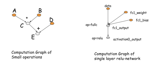
| First, let's revisit the idea of the computation graph. |
| A computation graph describes the (data flow) dependencies |
| between the operations in the deep network. |
| The operations performed in the graph |
| can be either fine-grained or coarse-grained. |
| The following figure shows two examples of computation graphs. |
| |
|  |
| |
| The concept of a computation graph is explicitly encoded in packages like Theano and CGT. |
| In other libraries, computation graphs appear implicitly as network configuration files. |
| The major difference in these libraries comes down to how they calculate gradients. |
| There are mainly two ways: performing back-propagation on the _same_ graph |
| or explicitly representing a _backwards path_ to calculate the required gradients. |
| |
| 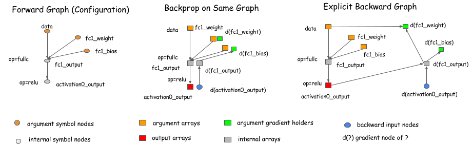 |
| |
| Libraries like Caffe, CXXNet, and Torch take the former approach, |
| performing back-prop on the original graph. |
| Libraries like Theano and CGT take the latter approach, |
| explicitly representing the backward path. |
| In this discussion, we adopt the *explicit backward path* approach |
| because it has several advantages for optimization. |
| |
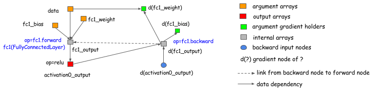
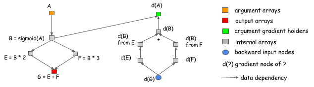
| However, we should emphasize that choosing the explicit backward path approach doesn't restrict us |
| to symbolic libraries, such as Theano and CGT. We can also use the explicit backward path for gradient calculation of |
| layer-based (which ties forward and backward together) libraries. The following graph shows how to do this. |
| Basically, we introduce a backward node that links to the forward node of the graph and calls the ```layer.backward``` |
| in the backward operations. |
| |
|  |
| |
| This discussion applies to almost all existing deep learning libraries. |
| (There are differences between libraries, e.g., higher-order differentiation, which is beyond the scope of this topic.) |
| |
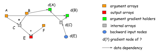
| Why is the explicit backward path better? Let's explain it with two examples. |
| The first reason is that the explicit backward path |
| clearly describes the dependency between computations. |
| Consider the following case, where we want to get |
| the gradient of A and B. As we can see clearly from the graph, |
| the computation of the ```d(C)``` gradient doesn't depend on F. |
| This means that we can free the memory of ```F``` |
| right after the forward computation is done. |
| Similarly, the memory of ```C``` can be recycled. |
| |
|  |
| |
| Another advantage of the explicit backward path |
| is the ability to have a different backward path, |
| instead of a mirror of forward one. |
| A common example is the split connection case, |
| as shown in the following figure. |
| |
|  |
| |
| In this example, the output of B is referenced by two operations. |
| If we want to do the gradient calculation in the same |
| network, we need to introduce an explicit split layer. |
| This means we need to do the split for the forward pass, too. |
| In this figure, the forward pass doesn't contain a split layer, |
| but the graph will automatically insert a gradient |
| aggregation node before passing the gradient back to B. |
| This helps us to save the memory cost of allocating the output of the split layer, |
| and the operation cost of replicating the data in the forward pass. |
| |
| If we adopt the explicit backward approach, |
| there's no difference between the forward pass and the backward pass. |
| We simply step through the computation graph in chronological order |
| and carry out computations. |
| This makes the explicit backward approach easy to analyze. |
| We just need to answer the question: |
| how do we allocate memory for each output node of a computation graph? |
| |
| |
| ## What Can Be Optimized? |
| |
| As you can see, the computation graph is a useful way |
| to discuss memory allocation optimization techniques. |
| Already, we've shown how you can save some memory |
| by using the explicit backward graph. |
| Now let's explore further optimizations, |
| and see how we might determine reasonable baselines for benchmarking. |
| |
| Assume that we want to build a neural network with `n` layers. |
| Typically, when implementing a neural network, |
| we need to allocate node space for both the output of each layer |
| and the gradient values used during back-propagation. |
| This means we need roughly `2 n` memory cells. |
| We face the same requirement when using the explicit backward graph approach |
| because the number of nodes in a backward pass |
| is roughly the same as in a forward pass. |
| |
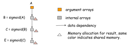
| ### In-place Operations |
| One of the simplest techniques we can employ |
| is _in-place memory sharing_ across operations. |
| For neural networks, we can usually apply this technique |
| for the operations corresponding to activation functions. |
| Consider the following case, where we want |
| to compute the value of three chained sigmoid functions. |
| |
|  |
| |
| Because we can compute sigmoid ```in-place```, |
| using the same memory for input and output, |
| we can compute an arbitrary-length chain |
| of sigmoid functions using constant memory. |
| |
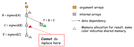
| Note: it's easy to make mistakes when implementing in-place optimization. |
| Consider the following case, where the value of B is used not only by C, but also by F. |
| |
|  |
| |
| We can't perform in-place optimization because the value of B |
| is still needed after ```C=sigmoid(B)``` is computed. |
| An algorithm that simply does in-place optimization |
| for every sigmoid operation might fall into such trap, |
| so we need to be careful about when we can use it. |
| |
| ### Standard Memory Sharing |
| In-place operations are not the only places where we can share memory. |
| In the following example, because the value of B is no longer needed |
| after we compute E, we can reuse B's memory to hold the result of E. |
| |
|  |
| |
| *Memory sharing doesn't necessarily require the same data shape*. |
| Note that in the preceding example, the shapes of `B` and `E` can differ. |
| To handle such a situation, we can allocate a memory region |
| of size equal to the maximum of that required by `B` and `E` and share it between them. |
| |
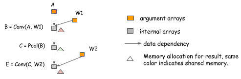
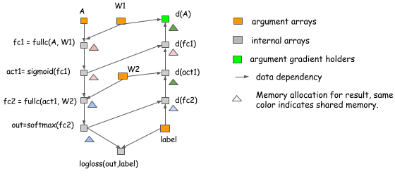
| ### Example of Real Neural Network Allocation |
| Of course, these are only toy examples and they address only the computation of the forward pass. |
| But the same ideas apply to real neural networks. |
| The following figure shows an allocation plan for a two-layer perceptron. |
| |
|  |
| |
| In this example: |
| |
| - In-place optimization is applied when computing ```act1```, ```d(fc1)```, ```out``` and ```d(fc2)```. |
| - Memory is shared between ```d(act1)``` and ```d(A)```. |
| |
| ## Memory Allocation Algorithm |
| |
| So far, we've discussed general techniques for optimizing memory allocation. |
| We've seen that there are traps to avoid, |
| as demonstrated in the case of in-place memory optimization. |
| So, how can we allocate memory correctly? |
| This is not a new problem. |
| For example, it is very similar |
| to the problem with register allocation in compilers. |
| There might be techniques that we can borrow. |
| We're not attempting to give a comprehensive review of techniques here, |
| but rather to introduce some simple |
| but useful tricks to attack the problem. |
| |
| The key problem is that we need to place resources |
| so that they don't conflict with each other. |
| More specifically, each variable has a *life time* |
| between the time it gets computed until the last time it is used. |
| In the case of the multi-layer perceptron, |
| the *life time* of ```fc1``` ends after ```act1``` get computed. |
| |
|  |
| |
| The principle is *to allow memory sharing only between variables whose lifetimes don't overlap*. |
| There are multiple ways to do this. |
| You can construct the conflicting graph |
| with each variable as a node and link the edge |
| between variables with overlapping lifespans, |
| and then run a graph-coloring algorithm. |
| This likely has ```$O(n^2)$``` complexity, |
| where ```n``` is the number of nodes in the graph. |
| This might be too costly. |
| |
| Let's consider another simple heuristic. |
| The idea is to simulate the procedure of traversing the graph, |
| and keep a count of future operations that depends on the node. |
| |
| 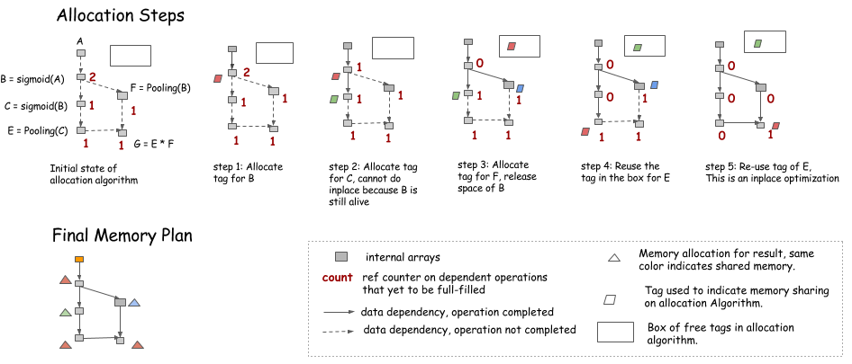 |
| |
| - An in-place optimization can be performed when only the current operation depends on the source (i.e., ```count==1```). |
| - Memory can be recycled into the box on the upper right corner when the ```count``` goes to 0. |
| - When we need new memory, we can either get it from the box or allocate a new one. |
| |
| ***Note:*** During the simulation, no memory is allocated. |
| Instead, we keep a record of how much memory each node needs, |
| and allocate the maximum of the shared parts in the final memory plan. |
| |
| ## Static vs. Dynamic Allocation |
| |
| The preceding strategy exactly simulates |
| the dynamic memory allocation procedure |
| in imperative languages, such as Python. |
| The ```count``` is the reference counter for each memory object, |
| and the object gets garbage collected |
| when the reference counter goes to 0. |
| In that sense, |
| we are simulating dynamic memory allocation once |
| to create a static allocation plan. |
| Can we simply use an imperative language |
| that dynamically allocates and deallocates memory? |
| |
| The major difference is that static allocation is only done once, |
| so we can afford to use more complicated algorithms. |
| For example, we can search for memory sizes |
| that are similar to the required memory block. |
| The Allocation can also be made graph aware. |
| We'll talk about that in the next section. |
| Dynamic allocation puts more pressure |
| on fast memory allocation and garbage collection. |
| |
| There is also one takeaway for users |
| who want to rely on dynamic memory allocations: |
| *do not unnecessarily reference objects*. |
| For example, if we organize all of the nodes in a list |
| and store then in a Net object, |
| these nodes will never get dereferenced, and we gain no space. |
| Unfortunately, this is a common way to organize code. |
| |
| |
| ## Memory Allocation for Parallel Operations |
| |
| In the previous section, we discussed |
| how we can *simulate* running the procedure |
| for a computation graph to get a static allocation plan. |
| However, optimizing for parallel computation presents other challenges |
| because resource sharing and parallelization are on the two ends of a balance. |
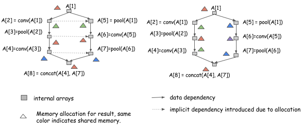
| Let's look at the following two allocation plans for the same graph: |
| |
|  |
| |
| Both allocation plans are valid |
| if we run the computation serially, |
| from ```A[1]``` to ```A[8]```. |
| However, the allocation plan on the left |
| introduces additional dependencies, |
| which means we can't run computation of ```A[2]``` and ```A[5]``` in parallel. |
| The plan on the right can. |
| To parallelize computation, we need to take greater care. |
| |
| ### Be Correct and Safe First |
| Being correct is our first principle. |
| This means to execute in a way that takes implicit dependency |
| memory sharing into consideration. |
| You can do this by adding the implicit dependency edge to the execution graph. |
| Or, even simpler, if the execution engine is mutation aware, |
| as described in [our discussion of dependency engine design](http://mxnet.io/architecture/note_engine.html), |
| push the operation in sequence |
| and write to the same variable tag |
| that represents the same memory region. |
| |
| Always produce a safe memory allocation plan. |
| This means never allocate the same memory |
| to nodes that can be parallelized. |
| This might not be ideal when memory reduction is more desirable, |
| and we don't gain too much when we can get benefit |
| from multiple computing streams simultaneously executing on the same GPU. |
| |
| ### Try to Allow More Parallelization |
| Now we can safely perform some optimizations. |
| The general idea is to try and encourage memory sharing between nodes that can't be parallelized. |
| You can do this by creating an ancestor relationship |
| graph and querying it during allocation, |
| which costs approximately ```$O(n^2)$``` in time to construct. |
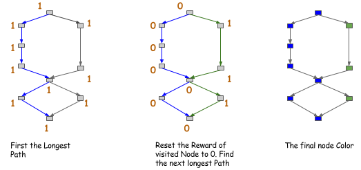
| We can also use a heuristic here, |
| for example, color the path in the graph. |
| As shown in the following figure, |
| when you try to find the longest paths in the graph, |
| color them the same color and continue. |
| |
|  |
| |
| After you get the color of the node, |
| you allow sharing (or encourage sharing) |
| only between nodes of the same color. |
| This is a stricter version of the ancestor relationship, |
| but it costs only `$O(n)$` of time |
| if you search for only the first `k` path. |
| |
| This is by no means the only solution. |
| More sophisticated approaches might exist: |
| |
| ## How Much Can you Save? |
| |
| We've discussed the techniques and algorithms you can use |
| to squeeze memory usage for deep learning. |
| How much can you really save by using these techniques? |
| |
| On coarse-grained operation graphs |
| that are already optimized for big operations, |
| you can reduce memory consumption roughly *by half*. |
| You can reduce memory usage even more |
| if you are optimizing a fine-grained computation network |
| used by symbolic libraries, such as Theano. |
| |
| Most of the ideas in this article inspired the design of _MXNet_. |
| We've also provided a [Memory Cost Estimation Script](https://github.com/dmlc/mxnet/tree/master/example/memcost), |
| which you can use to see how much memory you need under different scenarios. |
| |
| The script has an option called `forward_only`, |
| which shows the cost of running only the forward pass. |
| You will find that cost when using this option |
| is extremely low compared to others. |
| This is simply because there's more memory reuse |
| if you run only the forward pass. |
| |
| So here are two takeaways: |
| |
| - Use a computation graph to allocate memory. |
| - For deep learning models, prediction consumes much less memory than training. |
| |
| |
| ## Next Steps |
| |
| * [Efficient Data Loading Module for Deep Learning](http://mxnet.io/architecture/note_data_loading.html) |
| * [Survey of RNN Interface](http://mxnet.io/architecture/rnn_interface.html) |