Handwritten Digit Recognition

This tutorial guides you through a classic computer vision application: identify hand written digits with neural networks.

Loading Data

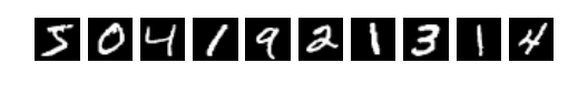
We first fetch the MNIST dataset, which is commonly used for handwritten digit recognition. Each image in this dataset has been resized into 28x28 with grayscale value between 0 and 254.

The following codes download and load the images and the according labels into memory.

import mxnet as mx
mnist = mx.test_utils.get_mnist()

using MXNet
include("mnist-data.jl")

require(mxnet)

xxx

Next we create data iterators for MXNet. A data iterator returns a batch of examples with according labels each time. If the examples are images, then they are represented by a 4-D matrix with shape (batch_size, num_channels, width, height). For the MNIST dataset, there is only one color channel, and both width and height are 28, therefore the shape is (batch_size, 1, 28, 28). In addition, we often shuffle the images used for training, which accelerates the training progress.

batch_size = 100
train_iter = mx.io.NDArrayIter(mnist['train_data'], mnist['train_label'], batch_size, shuffle=True)
val_iter = mx.io.NDArrayIter(mnist['test_data'], mnist['test_label'], batch_size)

batch_size = 100
train_provider, eval_provider = get_mnist_providers(batch_size)

Multilayer Perceptron

We first use multilayer perceptron to solve this problem. We define a multilayer perceptron by using MXNet's symbolic interface. The following command create a place holder variable for the input data.

data = mx.sym.var('data')
# Flatten the data from 4-D shape into 2-D (batch_size, num_channel*width*height)
data = mx.sym.flatten(data=data)

A multilayer perceptron contains several fully-connected layers. A fully-connected layer, with an n x m input matrix X outputs a matrix Y with size n x k, where k is often called as the hidden size. This layer has two learnable parameters, the m x k weight matrix W and the m x 1 bias vector b. It compute the outputs with Y = W X + b.

The output of a fully-connected layer is often feed into an activation layer, which performs element-wise operations. Common activation functions include sigmoid, tanh, and rectifier (or “relu”).

# The first fully-connected layer and the according activation function
fc1  = mx.sym.FullyConnected(data=data, num_hidden=128)
act1 = mx.sym.Activation(data=fc1, act_type="relu")

# The second fully-connected layer and the according activation function
fc2  = mx.sym.FullyConnected(data=act1, num_hidden = 64)
act2 = mx.sym.Activation(data=fc2, act_type="relu")

The last fully-connected layer often has the hidden size equals to the number of classes in the dataset. Then we stack a softmax layer, which map the input into a probability score. During the training stage, a cross entropy loss is then applied between the output and label.

# MNIST has 10 classes
fc3  = mx.sym.FullyConnected(data=act2, num_hidden=10)
# Softmax with cross entropy loss
mlp  = mx.sym.SoftmaxOutput(data=fc3, name='softmax')

# chain multiple layers with the mx.chain macro
mlp = @mx.chain mx.Variable(:data)             =>
  mx.FullyConnected(name=:fc1, num_hidden=128) =>
  mx.Activation(name=:relu1, act_type=:relu)   =>
  mx.FullyConnected(name=:fc2, num_hidden=64)  =>
  mx.Activation(name=:relu2, act_type=:relu)   =>
  mx.FullyConnected(name=:fc3, num_hidden=10)  =>
  mx.SoftmaxOutput(name=:softmax)

Now both the neural network definition and data iterators are ready. We can start training. The following commands train the multilayer perception on the MNIST dataset by minibatch (batch size is 100) stochastic gradient descent with learning rate 0.1. It stops after 10 epochs (data passes).

import logging
logging.getLogger().setLevel(logging.DEBUG)  # logging to stdout
# create a trainable module on CPU
mlp_model = mx.mod.Module(symbol=mlp, context=mx.cpu())
mlp_model.fit(train_iter,  # training data
              eval_data=val_iter,  # validation data
              optimizer='sgd',  # use SGD to train
              optimizer_params={'learning_rate':0.1},  # use fixed learning rate
              eval_metric='acc',  # report accuracy during training
              batch_end_callback = mx.callback.Speedometer(batch_size, 100), # output progress for each 100 data batches
              num_epoch=10)  # train at most 10 data passes

model = mx.FeedForward(mlp, context=mx.cpu())
optimizer = mx.SGD(lr=0.1, momentum=0.9, weight_decay=0.00001)
mx.fit(model, optimizer, train_provider, n_epoch=20, eval_data=eval_provider)

Convolutional Neural Networks

Note that the fully-connected layer simply reshapes the image into a vector during training. It ignores the spatial information that pixels are correlated on both horizontal and vertical dimensions. The convolutional layer aims to improve this drawback by using a more structural weight W. Instead of simply matrix-matrix multiplication, it uses 2-D convolution to obtain the output.

Besides the convolutional layer, another major change of the convolutional neural network is the adding of pooling layers. A pooling layer reduce a n x m patch into a single value to make the network less sensitive to the spatial location.

The following codes define a convolutional neural network called LeNet:

data = mx.sym.var('data')
# first conv layer
conv1 = mx.sym.Convolution(data=data, kernel=(5,5), num_filter=20)
tanh1 = mx.sym.Activation(data=conv1, act_type="tanh")
pool1 = mx.sym.Pooling(data=tanh1, pool_type="max", kernel=(2,2), stride=(2,2))
# second conv layer
conv2 = mx.sym.Convolution(data=pool1, kernel=(5,5), num_filter=50)
tanh2 = mx.sym.Activation(data=conv2, act_type="tanh")
pool2 = mx.sym.Pooling(data=tanh2, pool_type="max", kernel=(2,2), stride=(2,2))
# first fullc layer
flatten = mx.sym.flatten(data=pool2)
fc1 = mx.symbol.FullyConnected(data=flatten, num_hidden=500)
tanh3 = mx.sym.Activation(data=fc1, act_type="tanh")
# second fullc
fc2 = mx.sym.FullyConnected(data=tanh3, num_hidden=10)
# softmax loss
lenet = mx.sym.SoftmaxOutput(data=fc2, name='softmax')

# input
data = mx.Variable(:data)

# first conv
conv1 = @mx.chain mx.Convolution(data=data, kernel=(5,5), num_filter=20)  =>
mx.Activation(act_type=:tanh) =>
mx.Pooling(pool_type=:max, kernel=(2,2),
stride=(2,2))

# second conv
conv2 = @mx.chain mx.Convolution(data=conv1, kernel=(5,5), num_filter=50) =>
mx.Activation(act_type=:tanh) =>
mx.Pooling(pool_type=:max, kernel=(2,2), stride=(2,2))

# first fully-connected
fc1   = @mx.chain mx.Flatten(data=conv2) =>
mx.FullyConnected(num_hidden=500) =>
mx.Activation(act_type=:tanh)

# second fully-connected
fc2   = mx.FullyConnected(data=fc1, num_hidden=10)

# softmax loss
lenet = mx.Softmax(data=fc2, name=:softmax)

Now train LeNet with the same hyper-parameters as before. Note that, if GPU is available, it is desirable to use GPU for the computation given that LeNet is more complex than the previous multilayer perceptron. To do so, we only need to change mx.cpu() to mx.gpu().

# create a trainable module on GPU 0
lenet_model = mx.mod.Module(symbol=lenet, context=mx.cpu())
# train with the same
lenet_model.fit(train_iter,
                eval_data=val_iter,
                optimizer='sgd',
                optimizer_params={'learning_rate':0.1},
                eval_metric='acc',
                batch_end_callback = mx.callback.Speedometer(batch_size, 100),
                num_epoch=10)

# fit model
model = mx.FeedForward(lenet, context=mx.gpu())

# optimizer
optimizer = mx.SGD(lr=0.05, momentum=0.9, weight_decay=0.00001)

# fit parameters
mx.fit(model, optimizer, train_provider, n_epoch=20, eval_data=eval_provider)

Predict

After training is done, we can predict on new data. The following codes compute the predict probaility scores for every images, namely prob[i][j] is the probability that the i-th image contains the j-th object in the label set.

test_iter = mx.io.NDArrayIter(mnist['test_data'], None, batch_size)
prob = mlp_model.predict(test_iter)
assert prob.shape == (10000, 10)

If we have the labels for the new images, then we can compute the metrics.

test_iter = mx.io.NDArrayIter(mnist['test_data'], mnist['test_label'], batch_size)
# predict accuracy of mlp
acc = mx.metric.Accuracy()
mlp_model.score(test_iter, acc)
print(acc)
assert acc.get()[1] > 0.96

# predict accuracy for lenet
acc.reset()
lenet_model.score(test_iter, acc)
print(acc)
assert acc.get()[1] > 0.98