5分钟用MXNET上手神经网络

这是给初次使用mxnetR包的小白教程第一弹。你将学习到如何在5分钟内构件一个神经网络完成回归分析。

我们将想你展示如何分别执行分类任务和回归任务。这里的我们使用的数据来自 mlbench 包。

前言

本教程由Rmd编辑完成。

你可以直接访问主站版本的教程：MXNet R Document
你也可以从这里下载到Rmarkdown源文件

分类

首先，让我们加载数据并且做预处理：

require(mlbench)

## Loading required package: mlbench

require(mxnet)

## Loading required package: mxnet
## Loading required package: methods

data(Sonar, package="mlbench")

Sonar[,61] = as.numeric(Sonar[,61])-1
train.ind = c(1:50, 100:150)
train.x = data.matrix(Sonar[train.ind, 1:60])
train.y = Sonar[train.ind, 61]
test.x = data.matrix(Sonar[-train.ind, 1:60])
test.y = Sonar[-train.ind, 61]

下一步我们将用多层感知器作为分类器。在 mxnet 中，我们有一个mx.mlp函数，因此我们可以建立一个多层神经网络来做分类或者回归。

mx.mlp需要我们提供以下参数

训练数据和标签。
每个隐层的隐层节点数。
输出层的节点数。
激活函数类型。
数据损失函数类型。
计算引擎 (GPU 或者 CPU)。
其他给到 mx.model.FeedForward.create 的参数。

下面的代码段展示了mx.mlp的可能用法：

mx.set.seed(0)
model <- mx.mlp(train.x, train.y, hidden_node=10, out_node=2, out_activation="softmax",
                num.round=20, array.batch.size=15, learning.rate=0.07, momentum=0.9,
                eval.metric=mx.metric.accuracy)

## Auto detect layout of input matrix, use rowmajor..
## Start training with 1 devices
## [1] Train-accuracy=0.488888888888889
## [2] Train-accuracy=0.514285714285714
## [3] Train-accuracy=0.514285714285714
## [4] Train-accuracy=0.514285714285714
## [5] Train-accuracy=0.514285714285714
## [6] Train-accuracy=0.523809523809524
## [7] Train-accuracy=0.619047619047619
## [8] Train-accuracy=0.695238095238095
## [9] Train-accuracy=0.695238095238095
## [10] Train-accuracy=0.761904761904762
## [11] Train-accuracy=0.828571428571429
## [12] Train-accuracy=0.771428571428571
## [13] Train-accuracy=0.742857142857143
## [14] Train-accuracy=0.733333333333333
## [15] Train-accuracy=0.771428571428571
## [16] Train-accuracy=0.847619047619048
## [17] Train-accuracy=0.857142857142857
## [18] Train-accuracy=0.838095238095238
## [19] Train-accuracy=0.838095238095238
## [20] Train-accuracy=0.838095238095238

注意到在 mxnet中用来控制随机数种子的函数是 mx.set.seed. 你可以看到每一次迭代训练的准确性，这方便我们做预测和评估函数。

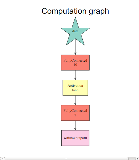
想要知道具体发生了什么，我们可以在R中轻松看到计算图：

graph.viz(model$symbol$as.json())

preds = predict(model, test.x)

## Auto detect layout of input matrix, use rowmajor..

pred.label = max.col(t(preds))-1
table(pred.label, test.y)

##           test.y
## pred.label  0  1
##          0 24 14
##          1 36 33

需要注意的是在多层预测中，mxnet输出矩阵是nclass x nexamples，每行都对应着每个类的概率。

回归

让我们先再一次做数据预处理。

data(BostonHousing, package="mlbench")

train.ind = seq(1, 506, 3)
train.x = data.matrix(BostonHousing[train.ind, -14])
train.y = BostonHousing[train.ind, 14]
test.x = data.matrix(BostonHousing[-train.ind, -14])
test.y = BostonHousing[-train.ind, 14]

虽然我们可以通过改变out_activation复用 mx.mlp 来做回归，这次我们还是会介绍一个弹性的方式来配置mxnet的神经网络。在mxnet中，这个配置通过“符号”系统来实现，这个系统将各个节点连接起来，比如激活、弃用比率等等。配置一个多层神经网络，我们可以通过下面的方式来完成：

# 定义输入数据
data <- mx.symbol.Variable("data")
# 一个全联通的隐层
# 数据: 输入源
# num_hidden: 隐层的神经节点数量
fc1 <- mx.symbol.FullyConnected(data, num_hidden=1)

# 每个输出层使用线性回归
lro <- mx.symbol.LinearRegressionOutput(fc1)

这让新网络可以优化方差损失。

上面的函数已经完成了回归的主要工作，我们现在可以在一个简单数据集上做训练。在这个配置中，我们弃用隐层，因此输入层是直接联通到输出层。

mx.set.seed(0)
model <- mx.model.FeedForward.create(lro, X=train.x, y=train.y,
                                     ctx=mx.cpu(), num.round=50, array.batch.size=20,
                                     learning.rate=2e-6, momentum=0.9, eval.metric=mx.metric.rmse)

## Auto detect layout of input matrix, use rowmajor..
## Start training with 1 devices
## [1] Train-rmse=16.063282524034
## [2] Train-rmse=12.2792375712573
## [3] Train-rmse=11.1984634005885
## [4] Train-rmse=10.2645236892904
## [5] Train-rmse=9.49711005504284
## [6] Train-rmse=9.07733734175182
## [7] Train-rmse=9.07884450847991
## [8] Train-rmse=9.10463850277417
## [9] Train-rmse=9.03977049028532
## [10] Train-rmse=8.96870685004475
## [11] Train-rmse=8.93113287361574
## [12] Train-rmse=8.89937257821847
## [13] Train-rmse=8.87182096922953
## [14] Train-rmse=8.84476075083586
## [15] Train-rmse=8.81464673014974
## [16] Train-rmse=8.78672567900196
## [17] Train-rmse=8.76265872846474
## [18] Train-rmse=8.73946101419974
## [19] Train-rmse=8.71651926303267
## [20] Train-rmse=8.69457600919277
## [21] Train-rmse=8.67354928674563
## [22] Train-rmse=8.65328755392436
## [23] Train-rmse=8.63378039680078
## [24] Train-rmse=8.61488162586984
## [25] Train-rmse=8.5965105183022
## [26] Train-rmse=8.57868133563275
## [27] Train-rmse=8.56135851937663
## [28] Train-rmse=8.5444819772098
## [29] Train-rmse=8.52802114610432
## [30] Train-rmse=8.5119504512622
## [31] Train-rmse=8.49624261719241
## [32] Train-rmse=8.48087453238701
## [33] Train-rmse=8.46582689119887
## [34] Train-rmse=8.45107881002491
## [35] Train-rmse=8.43661331401712
## [36] Train-rmse=8.42241575909639
## [37] Train-rmse=8.40847217331365
## [38] Train-rmse=8.39476931796395
## [39] Train-rmse=8.38129658373974
## [40] Train-rmse=8.36804269059018
## [41] Train-rmse=8.35499817678397
## [42] Train-rmse=8.34215505742154
## [43] Train-rmse=8.32950441908131
## [44] Train-rmse=8.31703985777311
## [45] Train-rmse=8.30475363906755
## [46] Train-rmse=8.29264031506106
## [47] Train-rmse=8.28069372820073
## [48] Train-rmse=8.26890902770415
## [49] Train-rmse=8.25728089053853
## [50] Train-rmse=8.24580511500735

这很容易做预测和评估。

preds = predict(model, test.x)

## Auto detect layout of input matrix, use rowmajor..

sqrt(mean((preds-test.y)^2))

## [1] 7.800502

现在，我们有4个预先定义的矩阵，分别是：“accuracy”, “rmse”, “mae” and “rmsle”. 你可能会对如何自定义评估矩阵感到困惑。mxnet 为自定义提供了一个接口：

demo.metric.mae <- mx.metric.custom("mae", function(label, pred) {
  res <- mean(abs(label-pred))
  return(res)
})

这里是一个平均绝对误差的一个例子。我们在一个训练函数中可以简单看看：

mx.set.seed(0)
model <- mx.model.FeedForward.create(lro, X=train.x, y=train.y,
                                     ctx=mx.cpu(), num.round=50, array.batch.size=20,
                                     learning.rate=2e-6, momentum=0.9, eval.metric=demo.metric.mae)

## Auto detect layout of input matrix, use rowmajor..
## Start training with 1 devices
## [1] Train-mae=13.1889538083225
## [2] Train-mae=9.81431959337658
## [3] Train-mae=9.21576419870059
## [4] Train-mae=8.38071537613869
## [5] Train-mae=7.45462437611487
## [6] Train-mae=6.93423301743136
## [7] Train-mae=6.91432357016537
## [8] Train-mae=7.02742733055105
## [9] Train-mae=7.00618194618469
## [10] Train-mae=6.92541576984028
## [11] Train-mae=6.87530243690643
## [12] Train-mae=6.84757369098564
## [13] Train-mae=6.82966501611388
## [14] Train-mae=6.81151759574811
## [15] Train-mae=6.78394182841811
## [16] Train-mae=6.75914719419347
## [17] Train-mae=6.74180388773481
## [18] Train-mae=6.725853071279
## [19] Train-mae=6.70932178215848
## [20] Train-mae=6.6928868798746
## [21] Train-mae=6.6769521329138
## [22] Train-mae=6.66184809505939
## [23] Train-mae=6.64754504809777
## [24] Train-mae=6.63358514060577
## [25] Train-mae=6.62027640889088
## [26] Train-mae=6.60738245232238
## [27] Train-mae=6.59505546771818
## [28] Train-mae=6.58346195800437
## [29] Train-mae=6.57285477783945
## [30] Train-mae=6.56259003960424
## [31] Train-mae=6.5527790788975
## [32] Train-mae=6.54353428422991
## [33] Train-mae=6.5344172368447
## [34] Train-mae=6.52557652526432
## [35] Train-mae=6.51697905850079
## [36] Train-mae=6.50847898812758
## [37] Train-mae=6.50014844106303
## [38] Train-mae=6.49207674844397
## [39] Train-mae=6.48412070125341
## [40] Train-mae=6.47650500999557
## [41] Train-mae=6.46893867486053
## [42] Train-mae=6.46142131653097
## [43] Train-mae=6.45395035048326
## [44] Train-mae=6.44652914123403
## [45] Train-mae=6.43916216409869
## [46] Train-mae=6.43183777381976
## [47] Train-mae=6.42455544223388
## [48] Train-mae=6.41731406417158
## [49] Train-mae=6.41011292926139
## [50] Train-mae=6.40312503493494

恭喜你！现在你已经学会如何基本使用mxnet。请查看其它教程学习更多高级功能。