TsFile 文件格式

1. TsFile 设计

本章是关于 TsFile 的设计细节。

1.1 变量的存储

数据类型
- 0: BOOLEAN
- 1: INT32 (int)
- 2: INT64 (long)
- 3: FLOAT
- 4: DOUBLE
- 5: TEXT (String)
编码类型
为了提高数据的存储效率，需要在数据写入的过程中对数据进行编码，从而减少磁盘空间的使用量。在写数据以及读数据的过程中都能够减少I/O操作的数据量从而提高性能。IoTDB支持多种针对不同类型的数据的编码方法：
- 0: PLAIN
  - PLAIN编码，默认的编码方式，即不编码，支持多种数据类型，压缩和解压缩的时间效率较高，但空间存储效率较低。
- 1: DICTIONARY
  - 字典编码是一种无损编码。它适合编码基数小的数据（即数据去重后唯一值数量小）。不推荐用于基数大的数据。
- 2: RLE
  - 游程编码，比较适合存储某些整数值连续出现的序列，不适合编码大部分情况下前后值不一样的序列数据。
  - 游程编码也可用于对浮点数进行编码，但在创建时间序列的时候需指定保留小数位数（MAX_POINT_NUMBER，具体指定方式参见SQL 参考文档）。比较适合存储某些浮点数值连续出现的序列数据，不适合存储对小数点后精度要求较高以及前后波动较大的序列数据。
    游程编码（RLE）和二阶差分编码（TS_2DIFF）对 float 和 double 的编码是有精度限制的，默认保留2位小数。推荐使用 GORILLA。
- 3: DIFF
- 4: TS_2DIFF
  - 二阶差分编码，比较适合编码单调递增或者递减的序列数据，不适合编码波动较大的数据。
- 5: BITMAP
- 6: GORILLA_V1
  - GORILLA编码是一种无损编码，它比较适合编码前后值比较接近的数值序列，不适合编码前后波动较大的数据。
  - 当前系统中存在两个版本的GORILLA编码实现，推荐使用GORILLA，不推荐使用GORILLA_V1（已过时）。
  - 使用限制：使用Gorilla编码INT32数据时，需要保证序列中不存在值为Integer.MIN_VALUE的数据点；使用Gorilla编码INT64数据时，需要保证序列中不存在值为Long.MIN_VALUE的数据点。
- 7: REGULAR
- 8: GORILLA

数据类型与支持编码的对应关系

数据类型	支持的编码
BOOLEAN	PLAIN, RLE
INT32	PLAIN, RLE, TS_2DIFF, GORILLA
INT64	PLAIN, RLE, TS_2DIFF, GORILLA
FLOAT	PLAIN, RLE, TS_2DIFF, GORILLA
DOUBLE	PLAIN, RLE, TS_2DIFF, GORILLA
TEXT	PLAIN, DICTIONARY

1.2 TsFile 概述

TsFile 整体分为两大部分：数据区和索引区。

数据区所包含的概念由小到大有如下三个：

Page 数据页：一段时间序列，是数据块被反序列化的最小单元；
Chunk 数据块：包含一条时间序列的多个 Page ，是数据块被 IO 读取的最小单元；
ChunkGroup 数据块组：包含一个实体的多个 Chunk。

索引区分为三部分：

按时间序列组织的 TimeseriesIndex，包含 1 个头信息和数据块索引（ChunkIndex）列表。头信息记录文件内某条时间序列的数据类型、统计信息（最大最小时间戳等）；数据块索引列表记录该序列各 Chunk 在文件中的 offset，并记录相关统计信息（最大最小时间戳等）；
IndexOfTimeseriesIndex，用于索引各 TimeseriesIndex 在文件中的 offset；
BloomFilter，针对实体（Entity）的布隆过滤器。

注：ChunkIndex 旧称 ChunkMetadata；TimeseriesIndex 旧称 TimeseriesMetadata；IndexOfTimeseriesIndex 旧称 TsFileMetadata。v0.13 版本起，根据其索引区的特性和实际所索引的内容重新命名。

下图是关于 TsFile 的结构图。

此文件包括两个实体 d1、d2，每个实体分别包含三个物理量 s1、s2、s3，共 6 个时间序列。每个时间序列包含两个 Chunk。

TsFile 的查询流程，以查 d1.s1 为例：

反序列化 IndexOfTimeseriesIndex，得到 d1.s1 的 TimeseriesIndex 的位置
反序列化得到 d1.s1 的 TimeseriesIndex
根据 d1.s1 的 TimeseriesIndex，反序列化其所有 ChunkIndex
根据 d1.s1 的每一个 ChunkIndex，读取其 Chunk 数据

1.2.1 文件签名和版本号

TsFile 文件头由 6 个字节的 “Magic String” (TsFile) 和 6 个字节的版本号 (000002) 组成。

1.2.2 数据区

ChunkGroup 数据块组

ChunkGroup 存储了一个实体 (Entity) 一段时间的数据。由若干个 Chunk, 一个字节的分隔符 0x00 和一个ChunkFooter组成。

Chunk 数据块

一个 Chunk 存储了一个物理量 (Measurement) 一段时间的数据，Chunk 内数据是按时间递增序存储的。Chunk 是由一个字节的分隔符 0x01, 一个 ChunkHeader 和若干个 Page 构成。

ChunkHeader 数据块头

成员	类型	解释
measurementID	String	传感器名称
dataSize	int	chunk 大小
dataType	TSDataType	chunk 的数据类型
compressionType	CompressionType	压缩类型
encodingType	TSEncoding	编码类型
numOfPages	int	包含的 page 数量

Page 数据页

一个 Page 页存储了一段时间序列，是数据块被反序列化的最小单元。它包含一个 PageHeader 和实际的数据 (time-value 编码的键值对）。

PageHeader 结构：

成员	类型	解释
uncompressedSize	int	压缩前数据大小
compressedSize	int	SNAPPY 压缩后数据大小
statistics	Statistics	统计量

这里是statistics的详细信息：

成员	描述	DoubleStatistics	FloatStatistics	IntegerStatistics	LongStatistics	BinaryStatistics	BooleanStatistics
count	数据点个数	long	long	long	long	long	long
startTime	开始时间	long	long	long	long	long	long
endTime	结束时间	long	long	long	long	long	long
minValue	最小值	double	float	int	long	-	-
maxValue	最大值	double	float	int	long	-	-
firstValue	第一个值	double	float	int	long	Binary	boolean
lastValue	最后一个值	double	float	int	long	Binary	boolean
sumValue	和	double	double	double	double	-	-

ChunkGroupFooter 数据块组结尾

成员	类型	解释
entityID	String	实体名称
dataSize	long	ChunkGroup 大小
numberOfChunks	int	包含的 chunks 的数量

1.2.3 索引区

1.2.3.1 ChunkIndex 数据块索引

第一部分的索引是 ChunkIndex ：

成员	类型	解释
measurementUid	String	传感器名称
offsetOfChunkHeader	long	文件中 ChunkHeader 开始的偏移量
tsDataType	TSDataType	数据类型
statistics	Statistics	统计量

1.2.3.2 TimeseriesIndex 时间序列索引

第二部分的索引是 TimeseriesIndex：

成员	类型	解释
measurementUid	String	物理量名称
tsDataType	TSDataType	数据类型
startOffsetOfChunkIndexList	long	文件中 ChunkIndex 列表开始的偏移量
ChunkIndexListDataSize	int	ChunkIndex 列表的大小
statistics	Statistics	统计量

1.2.3.3 IndexOfTimeseriesIndex 时间序列索引的索引（二级索引）

第三部分的索引是 IndexOfTimeseriesIndex：

成员	类型	解释
IndexTree	IndexNode	索引节点
offsetOfIndexArea	long	索引区的偏移量
bloomFilter	BloomFilter	布隆过滤器

索引节点 (IndexNode) 的成员和类型具体如下：

成员	类型	解释
children	List	节点索引项列表
endOffset	long	此索引节点的结束偏移量
nodeType	IndexNodeType	节点类型

索引项 (MetadataIndexEntry) 的成员和类型具体如下：

成员	类型	解释
name	String	对应实体或物理量的名字
offset	long	偏移量

所有的索引节点构成一棵类 B+树结构的索引树（二级索引），这棵树由两部分组成：实体索引部分和物理量索引部分。索引节点类型有四种，分别是INTERNAL_ENTITY、LEAF_ENTITY、INTERNAL_MEASUREMENT、LEAF_MEASUREMENT，分别对应实体索引部分的中间节点和叶子节点，和物理量索引部分的中间节点和叶子节点。只有物理量索引部分的叶子节点 (LEAF_MEASUREMENT) 指向 TimeseriesIndex。

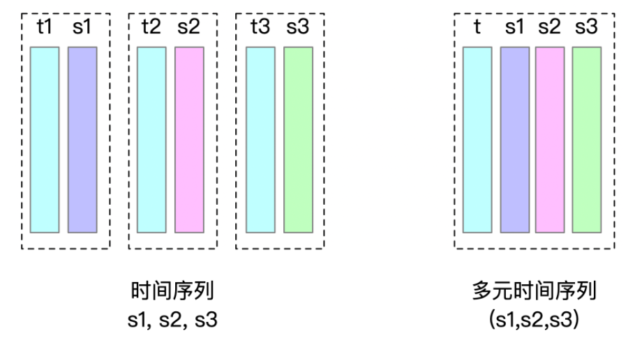
考虑多元时间序列的引入，每个多元时间序列称为一个vector，有一个TimeColumn，例如d1实体下的多元时间序列vector1，有s1、s2两个物理量，即d1.vector1.(s1,s2)，我们称vector1为TimeColumn，在存储的时候需要多存储一个vector1的Chunk。

构建IndexOfTimeseriesIndex时，对于多元时间序列的非TimeValue的物理量量，使用与TimeValue拼接的方式，例如vector1.s1视为“物理量”。

注：从0.13起，系统支持多元时间序列（Multi-variable timeseries 或 Aligned timeseries），一个实体的一个多元物理量对应一个多元时间序列。这些时间序列称为多元时间序列，也叫对齐时间序列。多元时间序列需要被同时创建、同时插入值，删除时也必须同时删除，一组多元序列的时间戳列在内存和磁盘中仅需存储一次，而不是每个时间序列存储一次。

下面，我们使用七个例子来加以详细说明。

索引树节点的度（即每个节点的最大子节点个数）可以由用户进行配置，配置项为max_degree_of_index_node，其默认值为 256。在以下例子中，我们假定 max_degree_of_index_node = 10。

需要注意的是，在索引树的每类节点（ENTITY、MEASUREMENT）中，键按照字典序排列。在下面的例子中，若i<j，假设字典序di<dj。（否则，实际上[d1,d2,...d10]的字典序排列应该为[d1,d10,d2,...d9]）

其中，例1~4为一元时间序列的例子，例5~6为多元时间序列的例子，例7为综合例子。

例 1：5 个实体，每个实体有 5 个物理量

在 5 个实体，每个实体有 5 个物理量的情况下，由于实体数和物理量数均不超过 max_degree_of_index_node，因此索引树只有默认的物理量部分。在这部分中，每个 IndexNode 最多由 10 个 IndexEntry 组成。根节点是 LEAF_ENTITY 类型，其中的 5 个 IndexEntry 指向对应的实体的 IndexNode，这些节点直接指向 TimeseriesIndex，是 LEAF_MEASUREMENT。

例 2：1 个实体，150 个物理量

在 1 个实体，实体中有 150 个物理量的情况下，物理量个数超过了 max_degree_of_index_node，索引树有默认的物理量层级。在这个层级里，每个 IndexNode 最多由 10 个 IndexEntry 组成。直接指向 TimeseriesIndex的节点类型均为 LEAF_MEASUREMENT；而后续产生的中间节点不是物理量索引层级的叶子节点，这些节点是 INTERNAL_MEASUREMENT；根节点是 LEAF_ENTITY 类型。

例 3：150 个实体，每个实体有 1 个物理量

在 150 个实体，每个实体中有 1 个物理量的情况下，实体个数超过了 max_degree_of_index_node，形成索引树的物理量层级和实体索引层级。在这两个层级里，每个 IndexNode 最多由 10 个 IndexEntry 组成。直接指向 TimeseriesIndex 的节点类型为 LEAF_MEASUREMENT，物理量索引层级的根节点同时作为实体索引层级的叶子节点，其节点类型为 LEAF_ENTITY；而后续产生的中间节点和根节点不是实体索引层级的叶子节点，因此节点类型为 INTERNAL_ENTITY。

例 4：150 个实体，每个实体有 150 个物理量

在 150 个实体，每个实体中有 150 个物理量的情况下，物理量和实体个数均超过了 max_degree_of_index_node，形成索引树的物理量层级和实体索引层级。在这两个层级里，每个 IndexNode 均最多由 10 个 IndexEntry 组成。如前所述，从根节点到实体索引层级的叶子节点，类型分别为INTERNAL_ENTITY 和 LEAF_ENTITY，而每个实体索引层级的叶子节点都是物理量索引层级的根节点，从这里到物理量索引层级的叶子节点，类型分别为INTERNAL_MEASUREMENT 和 LEAF_MEASUREMENT。

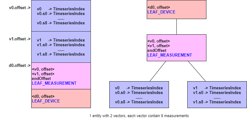
例 5：1 个实体，18 个物理量，2 个多元时间序列组，每个多元时间序列组分别有 9 个物理量

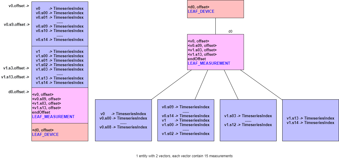
例 6：1 个实体，30 个物理量，2 个多元时间序列组，每个多元时间序列组分别有 15 个物理量

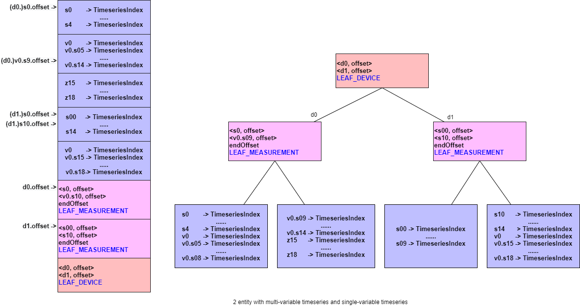
例 7：2 个实体，每个实体的物理量如下表所示

d0	d1
【一元时间序列】s0,s1...,s4	【一元时间序列】s0,s1,...s14
【多元时间序列】v0.(s5,s6,...,s14)	【多元时间序列】v0.(s15,s16,..s18)
【一元时间序列】z15,z16,..,z18

索引采用树形结构进行设计的目的是在实体数或者物理量数量过大时，可以不用一次读取所有的 TimeseriesIndex，只需要根据所读取的物理量定位对应的节点，从而减少 I/O，加快查询速度。有关 TsFile 的读流程将在本章最后一节加以详细说明。

1.2.4 Magic String

TsFile 是以 6 个字节的 magic string (TsFile) 作为结束。

恭喜您，至此您已经完成了 TsFile 的探秘之旅，祝您玩儿的开心！

2 TsFile 的总览图

v0.8

v0.9 / 000001

v0.10 / 000002

v0.12 / 000003

3 TsFile 工具集

3.1 IoTDB Data Directory 快速概览工具

该工具的启动脚本会在编译 server 之后生成至 server\target\iotdb-server-{version}\tools\tsfileToolSet 目录中。

使用方式：

For Windows:

.\print-iotdb-data-dir.bat <IoTDB 数据文件夹路径，如果是多个文件夹用逗号分隔> (<输出结果的存储路径>)

For Linux or MacOs:

./print-iotdb-data-dir.sh <IoTDB 数据文件夹路径，如果是多个文件夹用逗号分隔> (<输出结果的存储路径>)

在 Windows 系统中的示例：

D:\iotdb\server\target\iotdb-server-{version}\tools\tsfileToolSet>.\print-iotdb-data-dir.bat D:\\data\data
｜````````````````````````
Starting Printing the IoTDB Data Directory Overview
｜````````````````````````
output save path:IoTDB_data_dir_overview.txt
TsFile data dir num:1
21:17:38.841 [main] WARN org.apache.iotdb.tsfile.common.conf.TSFileDescriptor - Failed to find config file iotdb-engine.properties at classpath, use default configuration
|==============================================================
|D:\\data\data
|--sequence
|  |--root.ln.wf01.wt01
|  |  |--1575813520203-101-0.tsfile
|  |  |--1575813520203-101-0.tsfile.resource
|  |  |  |--device root.ln.wf01.wt01, start time 1 (1970-01-01T08:00:00.001+08:00[GMT+08:00]), end time 5 (1970-01-01T08:00:00.005+08:00[GMT+08:00])
|  |  |--1575813520669-103-0.tsfile
|  |  |--1575813520669-103-0.tsfile.resource
|  |  |  |--device root.ln.wf01.wt01, start time 100 (1970-01-01T08:00:00.100+08:00[GMT+08:00]), end time 300 (1970-01-01T08:00:00.300+08:00[GMT+08:00])
|  |  |--1575813521372-107-0.tsfile
|  |  |--1575813521372-107-0.tsfile.resource
|  |  |  |--device root.ln.wf01.wt01, start time 500 (1970-01-01T08:00:00.500+08:00[GMT+08:00]), end time 540 (1970-01-01T08:00:00.540+08:00[GMT+08:00])
|--unsequence
|  |--root.ln.wf01.wt01
|  |  |--1575813521063-105-0.tsfile
|  |  |--1575813521063-105-0.tsfile.resource
|  |  |  |--device root.ln.wf01.wt01, start time 10 (1970-01-01T08:00:00.010+08:00[GMT+08:00]), end time 50 (1970-01-01T08:00:00.050+08:00[GMT+08:00])
|==============================================================

3.2 TsFileResource 打印工具

该工具的启动脚本会在编译 server 之后生成至 server\target\iotdb-server-{version}\tools\tsfileToolSet 目录中。

使用方式：

Windows:

.\print-tsfile-resource-files.bat <TsFileResource 文件夹路径>

Linux or MacOs:

./print-tsfile-resource-files.sh <TsFileResource 文件夹路径>

在 Windows 系统中的示例：

D:\iotdb\server\target\iotdb-server-{version}\tools\tsfileToolSet>.\print-tsfile-resource-files.bat D:\data\data\sequence\root.vehicle
｜````````````````````````
Starting Printing the TsFileResources
｜````````````````````````
12:31:59.861 [main] WARN org.apache.iotdb.db.conf.IoTDBDescriptor - Cannot find IOTDB_HOME or IOTDB_CONF environment variable when loading config file iotdb-engine.properties, use default configuration
analyzing D:\data\data\sequence\root.vehicle\1572496142067-101-0.tsfile ...
device root.vehicle.d0, start time 3000 (1970-01-01T08:00:03+08:00[GMT+08:00]), end time 100999 (1970-01-01T08:01:40.999+08:00[GMT+08:00])
analyzing the resource file finished.

3.3 TsFile 描述工具

该工具的启动脚本会在编译 server 之后生成至 server\target\iotdb-server-{version}\tools\tsfileToolSet 目录中。

使用方式：

Windows:

.\print-tsfile-sketch.bat <TsFile 文件路径> (<输出结果的存储路径>)

注意：如果没有设置输出文件的存储路径，将使用 “TsFile_sketch_view.txt” 做为默认值。

Linux or MacOs:

./print-tsfile-sketch.sh <TsFile 文件路径> (<输出结果的存储路径>)

注意：如果没有设置输出文件的存储路径，将使用 “TsFile_sketch_view.txt” 做为默认值。

在 mac 系统中的示例：

/iotdb/server/target/iotdb-server-{version}/tools/tsfileToolSet$ ./print-tsfile-sketch.sh test.tsfile
｜````````````````````````
Starting Printing the TsFile Sketch
｜````````````````````````
TsFile path:test.tsfile
Sketch save path:TsFile_sketch_view.txt
-------------------------------- TsFile Sketch --------------------------------
file path: test.tsfile
file length: 15462
14:40:55.619 [main] INFO org.apache.iotdb.tsfile.read.TsFileSequenceReader - Start reading file test.tsfile metadata from 15356, length 96

            POSITION|	CONTENT
            -------- 	-------
                   0|	[magic head] TsFile
                   6|	[version number] 3
|||||||||||||||||||||	[Chunk Group] of root.sg_1.d1, num of Chunks:4
                   7|	[Chunk Group Header]
                    |		[marker] 0
                    |		[deviceID] root.sg_1.d1
                  21|	[Chunk] of s6, numOfPoints:1000, time range:[0,999], tsDataType:INT64, 
                     	startTime: 0 endTime: 999 count: 1000 [minValue:6,maxValue:9996,firstValue:6,lastValue:9996,sumValue:5001000.0]
                    |		[chunk header] marker=5, measurementId=s6, dataSize=1826, serializedSize=9
                    |		[chunk] java.nio.HeapByteBuffer[pos=0 lim=1826 cap=1826]
                    |		[page]  CompressedSize:1822, UncompressedSize:1951
                1856|	[Chunk] of s4, numOfPoints:1000, time range:[0,999], tsDataType:INT64, 
                     	startTime: 0 endTime: 999 count: 1000 [minValue:4,maxValue:9994,firstValue:4,lastValue:9994,sumValue:4999000.0]
                    |		[chunk header] marker=5, measurementId=s4, dataSize=1826, serializedSize=9
                    |		[chunk] java.nio.HeapByteBuffer[pos=0 lim=1826 cap=1826]
                    |		[page]  CompressedSize:1822, UncompressedSize:1951
                3691|	[Chunk] of s2, numOfPoints:1000, time range:[0,999], tsDataType:INT64, 
                     	startTime: 0 endTime: 999 count: 1000 [minValue:3,maxValue:9993,firstValue:3,lastValue:9993,sumValue:4998000.0]
                    |		[chunk header] marker=5, measurementId=s2, dataSize=1826, serializedSize=9
                    |		[chunk] java.nio.HeapByteBuffer[pos=0 lim=1826 cap=1826]
                    |		[page]  CompressedSize:1822, UncompressedSize:1951
                5526|	[Chunk] of s5, numOfPoints:1000, time range:[0,999], tsDataType:INT64, 
                     	startTime: 0 endTime: 999 count: 1000 [minValue:5,maxValue:9995,firstValue:5,lastValue:9995,sumValue:5000000.0]
                    |		[chunk header] marker=5, measurementId=s5, dataSize=1826, serializedSize=9
                    |		[chunk] java.nio.HeapByteBuffer[pos=0 lim=1826 cap=1826]
                    |		[page]  CompressedSize:1822, UncompressedSize:1951
|||||||||||||||||||||	[Chunk Group] of root.sg_1.d1 ends
|||||||||||||||||||||	[Chunk Group] of root.sg_1.d2, num of Chunks:4
                7361|	[Chunk Group Header]
                    |		[marker] 0
                    |		[deviceID] root.sg_1.d2
                7375|	[Chunk] of s2, numOfPoints:1000, time range:[0,999], tsDataType:INT64, 
                     	startTime: 0 endTime: 999 count: 1000 [minValue:3,maxValue:9993,firstValue:3,lastValue:9993,sumValue:4998000.0]
                    |		[chunk header] marker=5, measurementId=s2, dataSize=1826, serializedSize=9
                    |		[chunk] java.nio.HeapByteBuffer[pos=0 lim=1826 cap=1826]
                    |		[page]  CompressedSize:1822, UncompressedSize:1951
                9210|	[Chunk] of s4, numOfPoints:1000, time range:[0,999], tsDataType:INT64, 
                     	startTime: 0 endTime: 999 count: 1000 [minValue:4,maxValue:9994,firstValue:4,lastValue:9994,sumValue:4999000.0]
                    |		[chunk header] marker=5, measurementId=s4, dataSize=1826, serializedSize=9
                    |		[chunk] java.nio.HeapByteBuffer[pos=0 lim=1826 cap=1826]
                    |		[page]  CompressedSize:1822, UncompressedSize:1951
               11045|	[Chunk] of s6, numOfPoints:1000, time range:[0,999], tsDataType:INT64, 
                     	startTime: 0 endTime: 999 count: 1000 [minValue:6,maxValue:9996,firstValue:6,lastValue:9996,sumValue:5001000.0]
                    |		[chunk header] marker=5, measurementId=s6, dataSize=1826, serializedSize=9
                    |		[chunk] java.nio.HeapByteBuffer[pos=0 lim=1826 cap=1826]
                    |		[page]  CompressedSize:1822, UncompressedSize:1951
               12880|	[Chunk] of s5, numOfPoints:1000, time range:[0,999], tsDataType:INT64, 
                     	startTime: 0 endTime: 999 count: 1000 [minValue:5,maxValue:9995,firstValue:5,lastValue:9995,sumValue:5000000.0]
                    |		[chunk header] marker=5, measurementId=s5, dataSize=1826, serializedSize=9
                    |		[chunk] java.nio.HeapByteBuffer[pos=0 lim=1826 cap=1826]
                    |		[page]  CompressedSize:1822, UncompressedSize:1951
|||||||||||||||||||||	[Chunk Group] of root.sg_1.d2 ends
               14715|	[marker] 2
               14716|	[TimeseriesIndex] of root.sg_1.d1.s2, tsDataType:INT64
                    |		[ChunkIndex] s2, offset=3691
                    |		[startTime: 0 endTime: 999 count: 1000 [minValue:3,maxValue:9993,firstValue:3,lastValue:9993,sumValue:4998000.0]] 
               14788|	[TimeseriesIndex] of root.sg_1.d1.s4, tsDataType:INT64
                    |		[ChunkIndex] s4, offset=1856
                    |		[startTime: 0 endTime: 999 count: 1000 [minValue:4,maxValue:9994,firstValue:4,lastValue:9994,sumValue:4999000.0]] 
               14860|	[TimeseriesIndex] of root.sg_1.d1.s5, tsDataType:INT64
                    |		[ChunkIndex] s5, offset=5526
                    |		[startTime: 0 endTime: 999 count: 1000 [minValue:5,maxValue:9995,firstValue:5,lastValue:9995,sumValue:5000000.0]] 
               14932|	[TimeseriesIndex] of root.sg_1.d1.s6, tsDataType:INT64
                    |		[ChunkIndex] s6, offset=21
                    |		[startTime: 0 endTime: 999 count: 1000 [minValue:6,maxValue:9996,firstValue:6,lastValue:9996,sumValue:5001000.0]] 
               15004|	[TimeseriesIndex] of root.sg_1.d2.s2, tsDataType:INT64
                    |		[ChunkIndex] s2, offset=7375
                    |		[startTime: 0 endTime: 999 count: 1000 [minValue:3,maxValue:9993,firstValue:3,lastValue:9993,sumValue:4998000.0]] 
               15076|	[TimeseriesIndex] of root.sg_1.d2.s4, tsDataType:INT64
                    |		[ChunkIndex] s4, offset=9210
                    |		[startTime: 0 endTime: 999 count: 1000 [minValue:4,maxValue:9994,firstValue:4,lastValue:9994,sumValue:4999000.0]] 
               15148|	[TimeseriesIndex] of root.sg_1.d2.s5, tsDataType:INT64
                    |		[ChunkIndex] s5, offset=12880
                    |		[startTime: 0 endTime: 999 count: 1000 [minValue:5,maxValue:9995,firstValue:5,lastValue:9995,sumValue:5000000.0]] 
               15220|	[TimeseriesIndex] of root.sg_1.d2.s6, tsDataType:INT64
                    |		[ChunkIndex] s6, offset=11045
                    |		[startTime: 0 endTime: 999 count: 1000 [minValue:6,maxValue:9996,firstValue:6,lastValue:9996,sumValue:5001000.0]] 
|||||||||||||||||||||
               15292|	[IndexOfTimerseriesIndex Node] type=LEAF_MEASUREMENT
                    |		<s2, 14716>
                    |		<s6, 14932>
                    |		<endOffset, 15004>
               15324|	[IndexOfTimerseriesIndex Node] type=LEAF_MEASUREMENT
                    |		<s2, 15004>
                    |		<s6, 15220>
                    |		<endOffset, 15292>
               15356|	[TsFileMetadata]
                    |		[meta offset] 14715
                    |		[num of devices] 2
                    |		2 key&TsMetadataIndex
                    |		[bloom filter bit vector byte array length] 32
                    |		[bloom filter bit vector byte array] 
                    |		[bloom filter number of bits] 256
                    |		[bloom filter number of hash functions] 5
               15452|	[TsFileMetadataSize] 96
               15456|	[magic tail] TsFile
               15462|	END of TsFile
---------------------------- IndexOfTimerseriesIndex Tree -----------------------------
	[MetadataIndex:LEAF_DEVICE]
	└───[root.sg_1.d1,15292]
			[MetadataIndex:LEAF_MEASUREMENT]
			└───[s2,14716]
			└───[s6,14932]
	└───[root.sg_1.d2,15324]
			[MetadataIndex:LEAF_MEASUREMENT]
			└───[s2,15004]
			└───[s6,15220]]
---------------------------------- TsFile Sketch End ----------------------------------

3.4 TsFileSequenceRead

您可以使用示例中的类 example/tsfile/org/apache/iotdb/tsfile/TsFileSequenceRead 顺序打印 TsFile 中的内容。

3.5 Vis Tool

Vis 是一个把 TsFiles 中的 chunk 数据的时间分布以及点数可视化的工具。你可以使用这个工具来帮助你 debug，还可以用来观察数据分布等等。欢迎使用这个工具，在社区里交流你的想法。

图中的一个窄长矩形代表的是一个 TsFile 里的一个 chunk，其可视化信息为、[tsName, fileName, chunkId, startTime, endTime, pointCountNum]。
矩形在 x 轴上的位置是由该 chunk 的 startTime 和 endTime 决定的。
矩形在 y 轴上的位置是由以下三项共同决定的：
- (a)showSpecific: 用户指定要显示的特定时间序列集合。
- (b) seqKey/unseqKey 显示规则：从满足特定时间序列集合的 keys 提取 seqKey 或 unseqKey 时采取不同的显示规则：
  - b-1) unseqKey 识别 tsName 和 fileName，因此有相同 tsName 和 fileName 但是不同 chunkIds 的 chunk 数据将绘制在同一行；
  - b-2) seqKey 识别 tsName，因此有相同 tsName 但是不同 fileNames 和 chunkIds 的 chunk 数据将绘制在同一行，
- (c)isFileOrder：根据isFileOrder对 seqKey&unseqKey 进行排序，true 则以 fileName 优先的顺序排序， false 则以 tsName 优先的顺序排序。当在一张图上同时显示多条时间序列时，该参数将给用户提供这两种可选的观察视角。

3.5.1 如何运行 Vis

源数据包含两个文件：TsFileExtractVisdata.java和vis.m。 TsFileExtractVisdata.java从输入的 tsfile 文件中提取必要的可视化信息，vis.m用这些信息来完成作图。

简单说就是：先运行TsFileExtractVisdata.java然后再运行vis.m。

第一步：运行 TsFileExtractVisdata.java

TsFileExtractVisdata.java对输入的 tsfiles 的每一个 chunk 提取可视化信息 [tsName, fileName, chunkId, startTime, endTime, pointCountNum]，并把这些信息保存到指定的输出文件里。

该工具的启动脚本会在编译 server 之后生成至 server\target\iotdb-server-{version}\tools\tsfileToolSet 目录中。

使用方式：

Windows:

.\print-tsfile-visdata.bat path1 seqIndicator1 path2 seqIndicator2 ... pathN seqIndicatorN outputPath

Linux or MacOs:

./print-tsfile-visdata.sh path1 seqIndicator1 path2 seqIndicator2 ... pathN seqIndicatorN outputPath

参数：[path1 seqIndicator1 path2 seqIndicator2 ... pathN seqIndicatorN outputPath]

细节：

一共 2N+1 个参数。
seqIndicator：‘true’或者‘false’ （大小写不敏感）. ‘true’表示是顺序文件，‘false’表示是乱序文件。
Path：可以是一个 tsfile 的全路径，也可以是一个文件夹路径。如果是文件夹路径，你需要确保这个文件夹下的所有 tsfile 文件的seqIndicator都是一样的。
输入的所有 TsFile 文件必须是封好口的。处理未封口的文件留待未来有需要的情况再实现。

第二步：运行 vis.m

vis.m把TsFileExtractVisdata生成的 visdata 加载进来，然后基于 visdata 以及两个用户绘图参数showSpecific和isFileOrder来完成作图。

function [timeMap,countMap] = loadVisData(filePath,timestampUnit)
% Load visdata generated by TsFileExtractVisdata.
%
% filePath: the path of visdata.
% The format is [tsName,fileName,chunkId,startTime,endTime,pointCountNum].
% `tsName` and `fileName` are string, the others are long value.
% If the tsfile is unsequence file, `fileName` will contain "unseq" as an
% indicator, which is guaranteed by TsFileExtractVisdata.
%
% timestampUnit(not case sensitive):
%   'us' if the timestamp is microsecond, e.g., 1621993620816000
%   'ms' if it is millisecond, e.g., 1621993620816
%   's' if it is second, e.g., 1621993620
%
% timeMap: record the time range of every chunk.
% Key [tsName][fileName][chunkId] identifies the only chunk. Value is
% [startTime,endTime] of the chunk.
%
% countMap: record the point count number of every chunk. Key is the same
% as that of timeMap. Value is pointCountNum.

function draw(timeMap,countMap,showSpecific,isFileOrder)
% Plot figures given the loaded data and two plot parameters:
% `showSpecific` and `isFileOrder`.
%
% process: 1) traverse `keys(timeMap)` to get the position arrangements on
%          the y axis dynamically, which is defined simultaneously by
%           (a)`showSpecific`: traverse `keys(timeMap)`, filter out keys
%          that don't statisfy `showSpecific`.
%           (b) seqKey/unseqKey display policies: extract seqKey or unseqKey
%          from statisfied keys under different display policies:
%               b-1) unseqKey identifies tsName and fileName, so chunk data with the
%               same fileName and tsName but different chunkIds are
%               plotted on the same line.
%               b-2) seqKey identifies tsName, so chunk data with the same tsName but
%               different fileNames and chunkIds are plotted on the same
%               line.
%           (c)`isFileOrder`: sort seqKey&unseqKey according to `isFileOrder`,
%          finally get the position arrangements on the y axis.
%          2) traverse `keys(timeMap)` again, get startTime&endTime from
%          `treeMap` as positions on the x axis, combined with the
%          positions on the y axis from the last step, finish plot.
%
% timeMap,countMap: generated by loadVisData function.
%
% showSpecific: the specific set of time series to be plotted.
%               If showSpecific is empty{}, then all loaded time series
%               will be plotted.
%               Note: Wildcard matching is not supported now. In other
%               words, showSpecific only support full time series path
%               names.
%
% isFileOrder: true to sort seqKeys&unseqKeys by fileName priority, false
%              to sort seqKeys&unseqKeys by tsName priority.

3.5.2 例子

例 1

使用由IoTDBLargeDataIT.insertData写出的 tsfiles。小修改：IoTDBLargeDataIT.insertData最后添加一条statement.execute("flush");指令。

第一步：运行TsFileExtractVisdata.java

.\print-tsfile-visdata.bat data\sequence true data\unsequence false D:\visdata1.csv

或者等价地：

.\print-tsfile-visdata.bat data\sequence\root.vehicle\0\0\1622743492580-1-0.tsfile true data\sequence\root.vehicle\0\0\1622743505092-2-0.tsfile true data\sequence\root.vehicle\0\0\1622743505573-3-0.tsfile true data\unsequence\root.vehicle\0\0\1622743505901-4-0.tsfile false D:\visdata1.csv

第二步：运行vis.m

clear all;close all;

% 1. load visdata generated by TsFileExtractVisdata
filePath = 'D:\visdata1.csv';
[timeMap,countMap] = loadVisData(filePath,'ms'); % mind the timestamp unit

% 2. plot figures given the loaded data and two plot parameters:
% `showSpecific` and `isFileOrder`
draw(timeMap,countMap,{},false)
title("draw(timeMap,countMap,\{\},false)")

draw(timeMap,countMap,{},true)
title("draw(timeMap,countMap,\{\},true)")

draw(timeMap,countMap,{'root.vehicle.d0.s0'},false)
title("draw(timeMap,countMap,{'root.vehicle.d0.s0'},false)")

draw(timeMap,countMap,{'root.vehicle.d0.s0','root.vehicle.d0.s1'},false)
title("draw(timeMap,countMap,{'root.vehicle.d0.s0','root.vehicle.d0.s1'},false)")

draw(timeMap,countMap,{'root.vehicle.d0.s0','root.vehicle.d0.s1'},true)
title("draw(timeMap,countMap,{'root.vehicle.d0.s0','root.vehicle.d0.s1'},true)")

绘图结果：

附录

大端存储
- 比如： int 0x8 将会被存储为 00 00 00 08, 而不是 08 00 00 00
可变长的字符串类型
- 存储的方式是以一个 int 类型的 Size + 字符串组成。Size 的值可以为 0。
- Size 指的是字符串所占的字节数，它并不一定等于字符串的长度。
- 举例来说，“sensor_1” 这个字符串将被存储为 00 00 00 08 + “sensor_1” (ASCII编码)。
- 另外需要注意的一点是文件签名 “TsFile000001” (Magic String + Version), 因为他的 Size(12) 和 ASCII 编码值是固定的，所以没有必要在这个字符串前的写入 Size 值。
压缩类型
- 0: UNCOMPRESSED
- 1: SNAPPY
- 2: GZIP
- 3: LZO
- 4: SDT
- 5: PAA
- 6: PLA
- 7: LZ4