docs/observability/dogstack/trace.md

---
{
    "title": "Distributed Trace Analysis",
    "sidebar_label": "Traces",
    "language": "en-US",
    "description": "How do you analyze distributed traces in the Doris App? This article covers the trace scatter plot, waterfall view, Span Filter, and multi-dimensional filtering by service, operation, tags, and duration to help locate slow requests and abnormal calls.",
    "keywords": [
        "trace analysis",
        "distributed tracing",
        "Span Filter",
        "waterfall view",
        "Doris App",
        "Grafana",
        "OpenTelemetry",
        "slow request analysis"
    ]
}
---

<!-- Knowledge type: capability definition + operational steps -->
<!-- Applicable scenario: observability platform / distributed trace analysis -->

Trace is one of the three pillars of observability data. It tracks the full execution of a request and consists of spans — execution intervals within each service — and their call relationships. Traces are essential for analyzing request performance and anomalies in distributed systems.

You can analyze traces on the **Traces** page: locate the traces of interest (for example, long-running ones), then visualize a specific trace and drill into its spans.

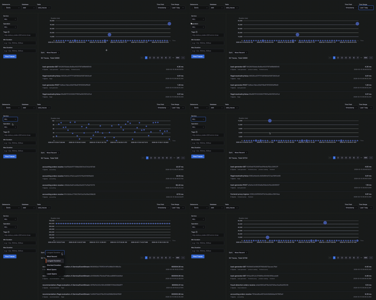
As shown below, the **Traces** page consists of four areas:

1. **Data selection area (top)**: Choose the trace data source (Datasource, Database, Table), time field, and time range.
2. **Filter area (left)**: Filter traces by Service, Operation, Tags, and Duration.
3. **Trace distribution area (top right)**: A scatter plot of matching traces — X-axis is trace start time, Y-axis is trace duration, and bubble size is the number of spans in the trace. The scatter plot helps you quickly spot long-running or large-span "big" traces. Click a bubble to view that trace's details as a waterfall chart.
4. **Trace list area (bottom right)**: A list of matching traces showing service, operation, trace_id, trace duration, span count, etc. The default sort `Most Recent` lists the newest traces by start time in descending order. You can switch the sort to show the longest/shortest traces or those with the most/fewest spans.

![Traces page overview](https://cdnd.selectdb.com/images/upload/dogstack/trace_page.gif)

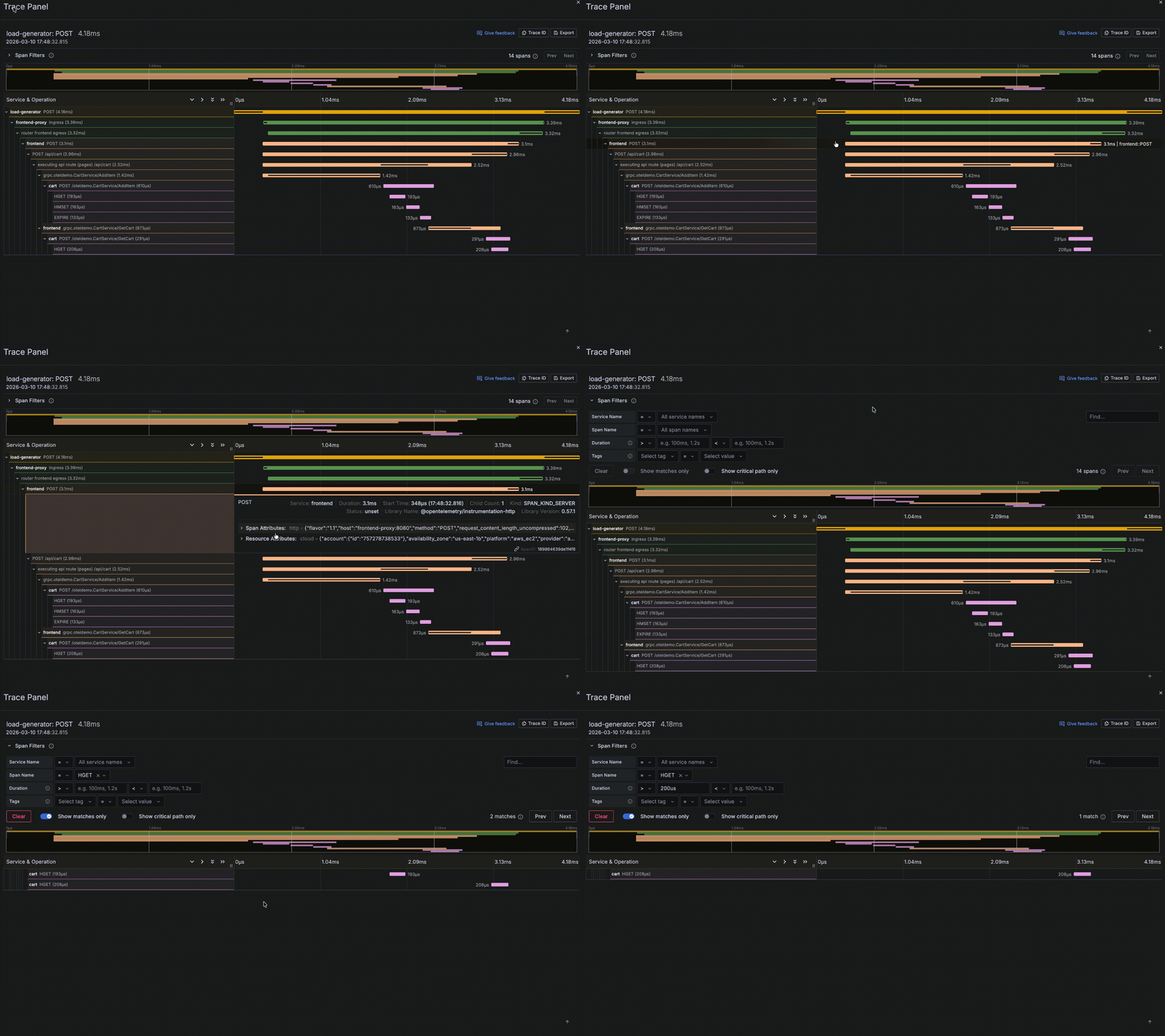
Clicking a trace opens a Trace Panel with rich details, where you can further analyze the spans in that trace:

1. View the trace's call-chain minimap and waterfall chart, including each span's execution window and call relationships.
2. Click a span to view its start time, duration, and contextual information including Span Attributes and Resource Attributes.
3. Click **Span Filter** to filter spans by Service Name, Span Name, Duration, Tags, etc.

![Trace Panel details](https://cdnd.selectdb.com/images/upload/dogstack/trace_panel.gif)



## Common filter examples

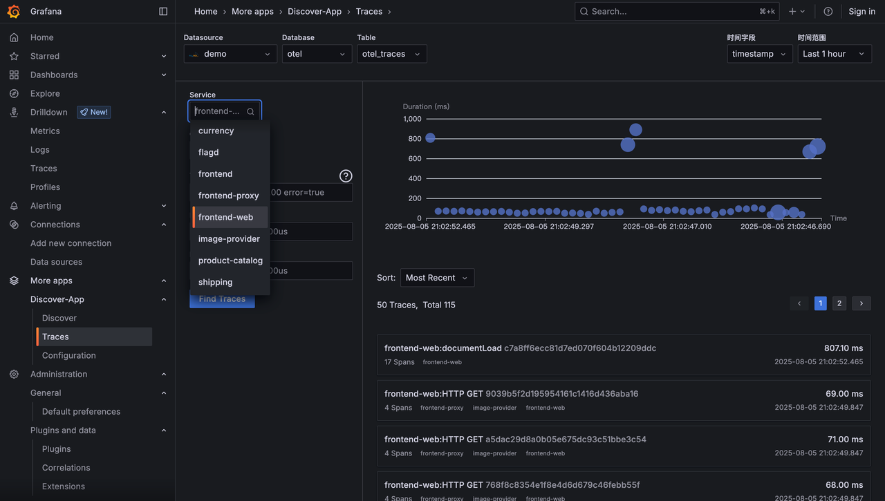
### Filter by service

```
Service = frontend-web
```

Quickly view traces produced by the specified service.

![Filter by service](https://cdnd.selectdb.com/images/upload/dogstack/trace_service.png)

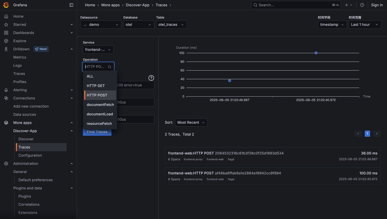
### Filter by operation

```
Operation = HTTP POST
```

Useful for locating a specific endpoint or request type.

![Filter by operation](https://cdnd.selectdb.com/images/upload/dogstack/trace_operation.png)

### Filter by tags

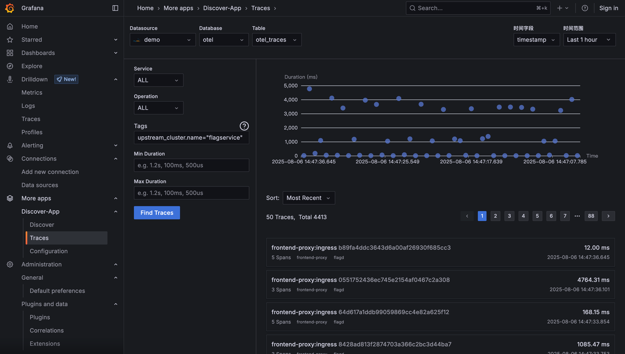
```
upstream_cluster.name="flagservice"
```

Use **logfmt key=value** syntax to filter on span attributes.

![Filter by tags](https://cdnd.selectdb.com/images/upload/dogstack/trace_tags.png)

### Filter by duration

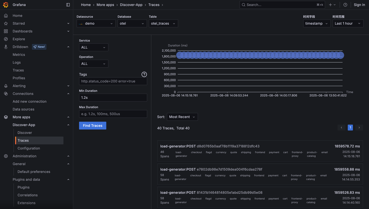
`Min Duration = 100ms ``Max Duration = 1.2s`

Quickly pinpoint slow requests.

![Filter by duration](https://cdnd.selectdb.com/images/upload/dogstack/trace_duration.png)



## Sorting and pagination

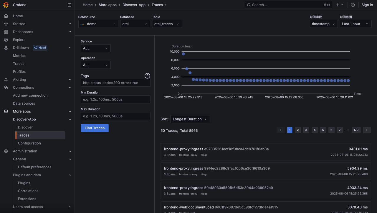
The trace list supports several sort options:

- Most Recent
- Longest / Shortest Duration
- Most / Fewest Spans

It also supports paginated browsing.

![Sorting and pagination](https://cdnd.selectdb.com/images/upload/dogstack/trace_sort.png)